Master Your Finances: Build a Simple Interactive Tracker in Excel or Google Sheets
Taking control of your money is one of the most vital life skills today. Whether it's budgeting for a vacation or managing monthly expenses, tracking your income and spending is key.
In this guide, you'll learn how to create an easy and effective, interactive income and expense tracker in Excel (or Google Sheets) that categorizes your finances and provides insightful reports. Best of all, this setup takes under 15 minutes, and once configured, it updates automatically!
![]()
Table of Contents
Watch the Excel Income & Expense Tracker Video

Get the Free Template
Too busy to build the Income & Expense Tracker yourself? Get the free template here and modify it for your needs:
Enter your email address below to download the sample workbook.

Step 1: Defining Categories
Your financial tracker begins with a clear structure of income and expense categories.
1. Create a Categories Sheet
- Start by listing your income and expense subcategories (e.g., "Groceries," "Salary").
- Organize them into larger groups (e.g., "Living Expenses," "Income Sources").
- Add a column to indicate whether each category is an income or an expense.
2. Format as a Table
- Use the shortcut CTRL+T to convert this list into an Excel table. This allows Excel to dynamically include new items when added.
3.Name and Style Your Table
- Rename the table to "Categories" for easy reference.
- Apply a light grey table style for clarity.
Your table should look like this, customised for your own categories and subcategories:
![]()
4. Set Up Subcategory for use in Data Validation
- Define a name for the subcategory column. Select the subcategories, then go to the Formulas tab > Define Name. This ensures dropdowns across the workbook (which we'll set up in a later step) update automatically with any changes.
(Note: Google Sheets users don't need to define a name.)
Step 2: Bank Transactions Table
Now, let's classify your bank transactions using your new categories.
1. Import Transaction Data
- Copy and paste data from your bank statements into a table. Include columns for date, description, debit, and credit.
- Add an "Account" column to track transactions from multiple accounts.
![]()
2. Categorize Transactions
- Insert a formula to calculate net values (Income - Expenses) for ease of reporting.
- Set up data validation to enable a dropdown list for selecting subcategories: Select subcategory column cells > Data tab > Data Validation > List. The Source is the defined name you created in the previous step for the subcategories column of the categories table:
![]()
- Select the subcategory for each transaction from the dropdown list:
![]()
3. Lookup Categories and Types
- Use XLOOKUP (or VLOOKUP) formulas to fetch the category and type based on the chosen subcategory.
![]()
4. Adding New Data
- Simply paste new transactions onto the next available row below the table. Excel's dynamic table feature will automatically include them, ensuring all linked formulas and references stay intact.
- Then select the subcategory for each transaction. More on updating the report later.
Step 3: Build Interactive Reports with PivotTables
With your data ready, it's time to create actionable insights - see video for step by step instructions for building the PivotTables.
- Income and Expense Reports
- Insert PivotTables to analyze income and expenses by category.
- Use Conditional Formatting to create visual data bars:
- Green for income (positive values).
- Pink for expenses (negative values).
- Hide text in bar chart columns using custom number formatting (;;;).
- Analyze Trends
- Group dates by year and month to display income or expenses over time.
- Copy PivotTables and adjust filters to show metrics like "Net Savings" or detailed breakdowns by subcategory.
- Dynamic Filtering with Slicers
- Add slicers for year and month to make filtering reports intuitive.
- Link slicers to specific PivotTables to streamline navigation.
Step 4: Create a Dashboard (optional)
For quick insights, design a professional dashboard:
- Add a header, such as "Income & Expenditure Dashboard."
- Display key metrics: total income, expenses, and net savings (PTD - Period to Date).
- Use Excel's GETPIVOTDATA function to reference PivotTable Income & Expense totals dynamically.
- Format as currency and add visual elements like icons for a polished look.
Your Income & Expense Tracker should look similar to this:
![]()
Step 5: Automating Updates
Updating your finance tracker is as simple as refreshing the data:
- Copy new transactions into the transactions table.
- Add the subcategories for each transaction.
- Go to the Data tab > Refresh All to update PivotTables and slicers automatically.
Smarter Decisions, Better Finances
This simple tracker is more than just a tool — it's a gateway to smarter financial decisions. By analyzing where your money goes each month, you can identify trends, cut unnecessary spending, and work toward your financial goals.
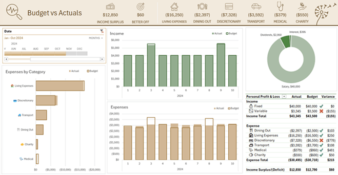
Next Steps: Controlling Your Budget
Ready to take control of your budget? Check out our Personal Budget in Excel guide to learn how to compare actual spending to budgeted goals for even greater control over your finances.
This Excel-based finance tracker is powerful, easy to maintain, and adaptable to your needs. Happy tracking!


Mynda,
Love your “Finance Tracker” (and your other tutorials.) I’ve not updated the tracker it in a while due to extensive travel schedule and now have an issue to cannot resolve. I’m trying to input new data (about 5 months worth) and when I start to type or paste anything (say the “Description”) the “Category” and “Category Type” both automatically change to #NAME?
I cannot seem to make these additions without getting the error. So I went back to the original file I file I purchased from you, and have found the same error. Has something changed? I use Microsoft Excel 365 (Excel Version 16.107.4) on my MacBook Air (OS 15.6.1).
Any pointers you can provide would be greatly appreciated.
Hi James,
The #NAME? error in Excel occurs when the formula contains text that Excel cannot recognise, usually due to typos in function names, undefined named ranges, missing quotation marks around text, or omitted colons in range references. Fix it by checking formula spelling, and references.
It could simply be that the version of Excel you are now using is old and doesn’t support the XLOOKUP function. You can test this in an empty cell, type =xl the formula IntelliSense list should display XLOOKUP, if it’s not listed, you have an old version of Excel that doesn’t support it.
That said, entering anything in the Description column won’t affect the Category and Category Type columns as they don’t reference it.
If you’re still stuck, please post your question on our Excel forum where you can also upload a sample file and we can help you further.
Mynda
P.S. the template was free. I never charge for templates 😉
Thank you for the tutorial and for providing the final product with the sample date. Very elegant design and functionality.
In preparation for replacing the sample date with my own, I deleted the November data from the transactions source table. Refreshing the data resulted in an error (#DIV/0!) in the upper row elements in the report tab. Interestingly, the upper left element (year/month) and the lower row elements work. I am pretty sure there are no blank rows in the data source. Any thoughts of how to fix this? Thank you.
Hi Gideon,
A #DIV! error means the denominator in the formula is zero. I suspect the cell the formula is referencing has changed/moved. You’re welcome to post your question on our Excel forum where you can also upload a sample file and someone can help you further.
Mynda
Why is it when i enter a blank entry or incorrect date format into the table the slicers for years and months disappear
There should never be blank rows in your transaction table. Just enter new data on the next available row below the table and it will automatically grow to include your data.
Blank rows result in the PivotTable not being able to determine the date for that row, which means it can’t group the dates, which means you can’t have Slicers for months. Likewise, if you enter a date in the incorrect format. See this tutorial on how to fix dates formatted as text if your dates need fixing into the correct date-serial number format.
Thank you.
That answer somewhat helped me. Im not sure I explained it clearly.So ill try again.
The downloaded template has the preloaded bank transactions. When I delete all the entires of the bank transactions from the table. To start fresh and add my own. The slicers used to filter year and month disappear. But,
When I delete all but the first entry in the table containing bank transactions. The slicers for years and months are still available. But if i were to add a new entry with an incorrect date format. The slicers for years and months than disappear. If I correct the date format and refresh the page. The slicers do not than return.
Understood. Don’t refresh the report until you have entered your data. If there’s no data to be grouped, then the PivotTable cannot support Slicers for months/years etc. Once the Slicers disappear, you have to insert them again and reconnect them to all the PivotTables. It’s easier just to delete my data, enter your own and only then, refresh the PivotTables. As long as your dates are entered correctly, the Slicers will remain intact.
hi,
I’m having an issue. i have a blank row in my transactions table if i put a data in this row and refresh my pivot tables. it messes them all up and my slicers disappear.
Hi Adam,
Remove the blank row. You should never have blank rows in your PivotTable source data. When you need to add new transactions, simply type or paste them in on the next blank row below the table and it will automatically expand to include the new data, you don’t need blank rows as placeholders ready to enter data.
Mynda
Thank you!
Glad it was helpful, Amo!
Thank you so much for providing this spreadsheet for us to use; much appreciated! My question: I’m 72, recently retired, and trying to understand how to tweak this for my use. I’ve entered my YTD info into the Transactions tab and like the results I see on the Report tab. Selecting different months (or years) to see the specific info is very cool. What I would like to also see is a difference between a “budgeted” amount for each category, as well as the spending MTD for that category. This would enable me to see each category’s ongoing balance for the month (even if the result is zero or negative). Am I being clear in my question? How would I go about this. I’ve used Excel for years, but very basically – no Pivot Table usage….
Thanks / Dan
Hi Dan,
Glad it was helpful. See this Personal Budget Tracker spreadsheet for incorporating a budget component.
Mynda
Hi Mynda,
I just downloaded the Personal Budget Tracker spreadsheet and it looks great; I’ll start massaging it for my categories and transactions. What a helpful group of tools you’re providing for people. Much thanks!
Dan
Awesome to hear, Dan!
Is this doable in Google Sheets I Tried but most of the features are not available
Yes, but you will have to lookup how to insert conditional formatting data bars in Sheets, as the process is different.
Really grateful for such a useful application and intro to revisiting vlookup, etc. How much work would be involved in showing not only a particular year’s monthly income and expenses, but also displaying perious years’ monthly totals to compare how income/expenses is tracking for similar periods of the year, year on year? In line graph form?
Hi John,
You can certainly include prior years’ data, as for how much work that would involve, that depends on how many transactions you have as you’d have to enter at least monthly totals by category.
Mynda
Hi, I have been trying to delete the template data for 2025 and input my own but I am struggling to do this. Whenever I delete the data and put my own data in it gets rid of all the data from the report tab. Any advice on how to remedy this would be greatly appreciated. Many thanks!
It will be one of three things:
1. You have filters applied that exclude your data e.g. filtered for 2025 and you only have data for 2026 etc.
2. You have changed the names of the columns in the transaction table, so the PivotTables no longer see the columns they were originally set up with.
3. Your dates are not entered in a correct date format that Excel can interpret. e.g. you’ve entered them as text.
You’re welcome to post your question on our Excel forum where you can also upload an Excel file and we can help you further.
Is it possible to split a transaction between several expense categories?
Yes, just enter the same date and transaction number/ID and split the amounts according to the expense categories you want to assign.
How do I add a new value in the “Account” drop down? I would like to be able to track my paycheck deductions also. Thanks!
In the Bank Transactions table there is no drop-down in the ‘Account’ column. You can just type in a new account name, then when you ‘Refresh All’ (on the Data tab), the account type will be available in the filters.
Hi Mynda, I have excel 2010… are there any features you are using that are not in this version?
I just downloaded the template and it loaded and seems to function
Thanks
Hi John,
The ‘Tracker’ sheet will work in 2010, but the ‘Schedule’ sheet won’t be possible. The minute you edit those formulas, they will return errors because you don’t have the SORT, FILTER or SEQUENCE functions.
Mynda
Hi Mynda Treacy! Really impressed by the work you have made. I feel, it is very useful and I have planned to implement it for my personal budgeting and expense tracking use.
Moreover, could I ask a favour, could you walk me through how to make the report sheet in google sheets? For instance, all the features such as data bar, slicer in google sheet. It is clear to use in excel but in google sheets how do I acheive?
Thank you!
Glad you found it useful, Sam. I don’t use Google Sheets, so I can’t point you to any tutorials, sorry.
Hello!
I found your video on YouTube, and I wanted to create an Excel file with my categories, but I don’t have the XLOOKUP function, and I’m unsure how to use VLOOKUP for this purpose.
Except for the “account” column, the table remains the same; only the names differ.
How should the VLOOKUP formula look?
Thank you!
Please see this tutorial on how to use VLOOKUP. If you get stuck, please post your question on our Excel forum where you can also upload a sample file and we can help you further.
Hi Mynda,
thanks for the template & explanation! Could you explain if it’s possible to add data from multiple sheets to the pivot tables on the report sheet?
i.e. if I have one sheet per year, that is, one sheet with all expenses + income from 2025, one from 2024, etc.
Thanks, Elena
Hi Elena,
You should never split your source data over multiple sheets. This prevents you using the Excel tools the way they were intended. I recommend keeping it all in one sheet and add a column for the date. You can then use the PivotTables and Slicers to filter the report to show the years you want.
Mynda
Great job. Thanks
Glad you liked it!
How can I get the Category and Category Type to populate on the Bank Transactions tab. It just says, “#NAME”
thank you
The #NAME? error in Excel means the formula contains text Excel doesn’t recognize, often due to a misspelled function or named range, missing text quotation marks, or using a new function in an old Excel version. You’re welcome to post your question on our Excel forum where you can also upload a sample file and we can help you further.
Hello!
This is extremely helpful, thank you for your time and efforts! Is there a way to enter a starting balance for checking/savings/investing accounts?
Great to hear. You can enter the opening balance as the first transaction in your transactions table.
Hi Mynda
Thank you, this is fantastic. i followed your steps in the video to create the template. but i notice that when i press refresh I’m losing my dates in the pivottable fields and the slicers disappear. Any idea where i might have gone wrong and why
Glad it was helpful, Gary. It sounds like a date issue. My dates are dd/mm/yyyy and your dates are probably mm/dd/yyyy. You will need to make sure the date format for your date cells is mm/dd/yyyy (select the cells, CTRL+1 to open the formatting pane, select the number format tab, under ‘date’, select your date format).
Then check your dates are displaying correctly. You may need to enter them again.
Then refresh the PivotTables. You may need to remove and re-add the date field. Then select any date cell in a PivotTable > right-click > group. Group by month and year.
If you’re still stuck, please post your question on our Excel forum where you can also upload your Excel file and we can help you further.
Mynda
Dear Mynda,
I saw the Youtube video and I was stoked. Thank you for the great work. I downloaded the template, deleted the example data and entered my own data. One question, and one problem:
1. What is the difference between the Bank Transactions and the Nov Data sheets? Is the Nov Data sheet for transactions that are not bank transactions? Why use different sheets? Do the pivot table aggregate the results from both sheets?
2. I get an error message when I update the pivot tables: “The action for the “PivotTable9” in the “Report” sheet could not be completed because there is already a PivotTable “PivotTable 13”. Free up memory and try again.” (This is a translation as I am using the German Excel version). Any idea how to fix this? Google and ChatGPT did not help. I tried the tracker on an 8GB Mac and a 16GB Windows machine. Same error.
Thanks, Daniel
Hi Daniel,
That error is because PivotTable 9 wants to insert more rows, but there are PivotTables in the way. Insert some empty rows below PivotTable 9 to allow it enough space.
Mynda
Thankyou
Glad you liked it, Bryan.
Is the current downloadable template in early 2025 the same as the 2024 template, or have you made substantial updates? I found the 2024 file very useful.
Hi Scott,
This uses a completely different approach. i.e. no Power Query to manipulate the data and no budget comparison.
Mynda
The Income and Expense Categories are understood.
What is proposed for Capital transactions?
e.g. Asset Purchases, Loan Repayments?
Regards, Roger H
Hi Roger,
You can add categories for assets and liabilities, and an additional PivotTable to track them.
Mynda
Thank you very much for sending updates via email. I found every excel template sent by you, very useful and I learned to love excel more than any other Microsoft office programs. Now, excel is my favorite and handy program on a daily basis working schedule.
My warm regards to all your team
Leila
Awesome to hear, Leila!
Thank you
Our pleasure!