Good morning, Forum
I am asking for your help (again please) with an issue I have using Power Pivot / Data Model and creating measures.
I have a column with the end date of a course, a column with the return date of the documentation for this course and a column calculating the days taken. If there is no return date, I have calculated a blank cell using "" in the IF statement. Formula as follows.
=IF([@[File Return Date]]="","",NETWORKDAYS([@[End Date]],[@[File Return Date]])-1)
My problem seems to arise with the handling of the blank cells. Having used "" to represent the blank cells Power Pivot will only format the data as text which in turn means I cannot create any measures to use in graphical representations. I have tried using the ‘BLANK()’ option but must confess I am struggling a little to make this work.
If you have any ideas or suggestions – that would be most appreciated.
Many thanks in advance.
Rachel 
You either need to calculate workdays within PP (different options to be found on-line) as PP doesn't recognize NETWORKDAYS or you can use a workaround.
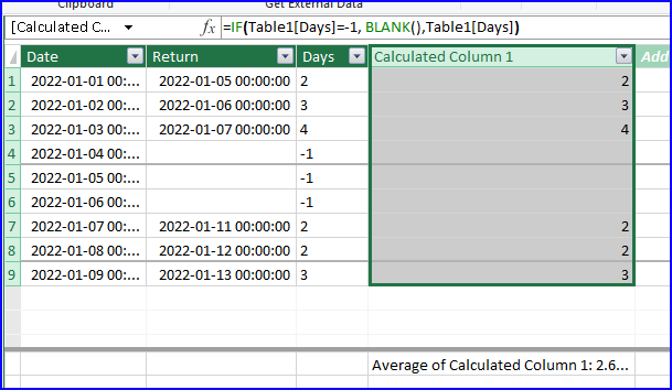
Change your formula in Excel to return a value, let's say -1, rather than an empty string "". Call it Days, for instance.
Then, in PP add a calculated column with a formula similar to this:
=IF(Table1[Days]=-1, BLANK(),Table1[Days])
Now you end up with a column containing numbers and blanks that can be used in measures.

Apologies, I have just realised there are some key points to note that I have omitted...
- The use of icon sets in conditional formatting
- In the formula above, I have considered replacing "" with 0, but there are instances were paperwork is returned the same day and therefore the lag between the two is 0 days
I have attached a spreadsheet as an example of where we are. We now need the ability to interrogate the data further, hence popping the data into the data model and producing pivot charts on a dashboard.
Thanks again in advance.
Kind regards
Rachel 
You can still return -1 in stead of "", but you would have to change the formula like the one in H2 to:
=COUNTIF(Table1[FRD Days],">=0")
and the one in H3 to:
=COUNTIFS(Table1[FRD Days],"<=3",Table1[FRD Days],">=0")
With regard to not showing CF icons for cells with the -1 values, add an initial CF rule that returns the value with a custom number format ";;" when there is no date in column G (i.e. don't display the number at all) and mark it Stop if true.
Done all that in the attached file (column H only).
Wow! That's amazing.. it works perfectly!
Thank you so much for your guidance Riny - it is very mcuh appreciated. 
