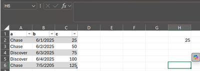
Hi,
I have this sample spreadsheet where I am trying to search in a table by name in column A, then search by date range in column B then add the total from column C.
I am looking for "Chase" in column A, then search in column B from 6/1/2025 through 6/3/2025 and finally add up the sum in column C.
Copilot gave me this formula: =SUMIFS(C2:C100, A2:A100, "Chase", B2:B100, ">=6/1/2025", B2:B100, "<=6/3/2025")
Instead of giving the value of 75, it has 25?
Also I will have this value on sheet1, would {sheet1
!} be in front of the formula?
Thanks!
Okay, I used ChatGPT which said to use this more reliable date function =SUMIFS(C2:C6, A2:A6, "Chase", B2:B6, ">="&DATE(2025,6,1), B2:B6, "<="&DATE(2025,6,3)).
It then told me to check the names in Column A by using =LEN(A3), which showed an error.
With Power Query. The hard coded filters could be parameter queries if you are looking for more variables in your lookups.
let
Source = Excel.CurrentWorkbook(){[Name="Table1"]}[Content],
#"Changed Type" = Table.TransformColumnTypes(Source,{{"b", type date}}),
#"Filtered Rows" = Table.SelectRows(#"Changed Type", each ([a] = "Chase")),
#"Filtered Rows1" = Table.SelectRows(#"Filtered Rows", each [b] >= #date(2025, 6, 1) and [b] <= #date(2025, 6, 3)),
#"Grouped Rows" = Table.Group(#"Filtered Rows1", {"a"}, {{"Total", each List.Sum([c]), type number}})
in
#"Grouped Rows"
Cell A3 contains "Chase " (note the trailing space!). SUMIF is looking for "Chase" and thus skips the value for "Chase ". Remove the space and your formula will work.
And I would indeed use the ChatGPT suggested formula with the DATE function. Hardcoding the date in the m/d/yyyy format will work for you but not for users on a system with a different date setting. For example like dd/mm/yyyy or yyyy-mm-dd.

