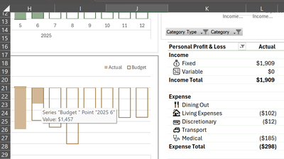
I am using a top row to add the totals for certain items. Right now I'm using a simple reference =L28, which is the Expense Total that equals ($298) The problem is that when I want to remove Transport, the cell location changes.
I'm trying to use GETPIVOTDATA to extract that but I keep on getting errors on the formula. The Pivot table is called PTProfitLoss.
I've tried variations of =GETPIVOTDATA("Actual",$A$3,"Category","Expense Total") that was generated by AI. However I keep getting errors.
Any suggestions.
Thanks
The template you are using (Mynda's) has rectangle shapes that contain the references to individual cells inside pivot tables. Such shapes can not contain formulas with functions like GETPIVOTDATA. You need to create such references somewhere else in the workbook. I suggest in the Analytics sheet, similar to what you see in C2 and C3 in that sheet. These cells are referenced by the first to rectangles in the Report header.
Based on the original template the following formula will pick-up the correct cell for Total Expenses:
=GETPIVOTDATA("Actual ",$K$16,"Category Type","Expense")

