Hello,
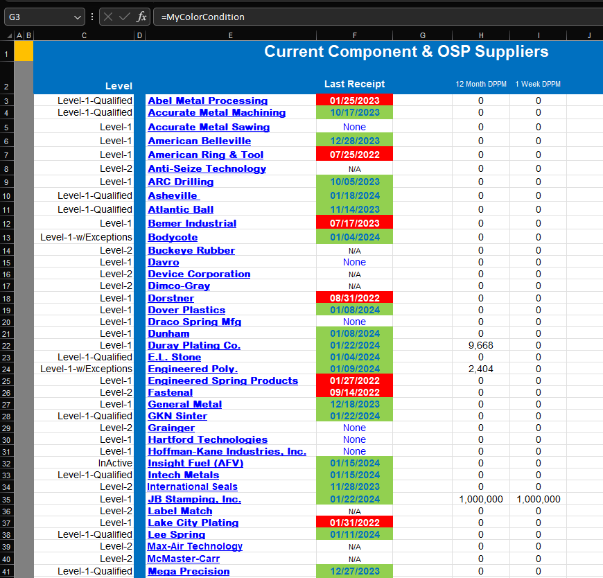
I am looking for a formula to automatically fill Cells with the words "Send to QA" when the adjacent cell to the left turns red based on the conditional formatting for those cells.
I have defined the name -- MyColorConditon and used this formula:
=IF(GET.CELL(38,INDEX!$F$3)=10,"No",IF(GET.CELL(38,INDEX!$F$3)=3,"Send to QA",""))
I Set cell G3 =MyColorCondition and nothing happens.
I need a formula that I don't need to define the name. It is not a macro enabled book and don't want to make it one.
![]()

Get.cell does not recognise conditional formatting & even if it did you would need to save the workbook as macro enabled.
The simplest thing is to use the criteria from the CF for your formula, along the lines of
=if(f3<edate(today(),-6),"Send to QA","")
Hello Fluff,
When I enter this into my workbook, all I get is a 0.![]()
Hello,
You do probably have the advanced setting set to show a 0 (zero) for null values.
If not, please share your file (do remove sensitive data first) so we can help you out better.
Br,
Anders
That formula is pointing to itself & so creating a circular reference.
In your original image the dates were in col F, now they are in col E so it should be
=if(e3<edate(today(),-6),"Send to QA","")
Thank you Fluff. That worked. Is there a way to not show "Send to QA" in the fields where there are no records yet?
How about
=IF(OR(E3>EDATE(TODAY(),-6),E3=""),"","Send to QA")
Hello Fluff,
That worked. Thank you for all the help.
Have a great day!
