
Most Excel users know the basics like Ctrl+C, Ctrl+V, and maybe Ctrl+D.
But there are shortcuts that go far beyond that. Some save small amounts of time. Others remove frustrating roadblocks entirely.
In this guide, you’ll learn 12 powerful Excel shortcuts that most people never discover, even after years of using Excel.
Table of Contents
- See the Hidden Excel Shortcuts in Action
- Get the Example File
- Shortcut 1: Ctrl + Shift + U
- Shortcut 2: Ctrl + J
- Shortcut 3: Alt + Enter
- Shortcut 4: F2 (it’s not what you think)
- Shortcut 5: Ctrl + Backspace
- Shortcut 6: Tab (this isn’t what you think either)
- Shortcut 7: Ctrl + .
- Shortcut 8: Ctrl + Drag Sheet Tab
- Shortcut 9: Ctrl + Click Sheet Navigation Arrows
- Shortcut 10: Shift + Scroll
- Shortcut 11: F3
- Shortcut 12: F4 (not for absolute references)
- Take Your Excel Skills Further
See the Hidden Excel Shortcuts in Action

Get the Example File
Enter your email address below to download the free file.

Shortcut 1: Ctrl + Shift + U
Working with long formulas can be painful when you only see one line at a time in the formula bar.
Many users manually drag the formula bar or click the expand button. Both approaches interrupt your workflow.
Press Ctrl + Shift + U to instantly expand the formula bar so you can view the entire formula.
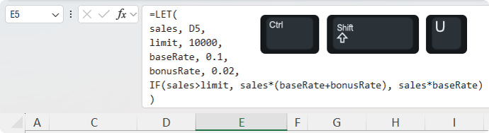
Press it again to collapse it.
This is especially useful when working with LET or LAMBDA formulas where readability matters.
Shortcut 2: Ctrl + J
If your column headers contain long dates, they can make your worksheet unnecessarily wide as shown in the image below:
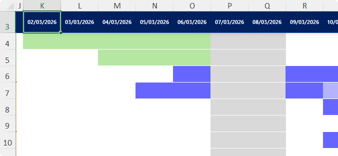
Instead, you can split the date across two lines using a custom format.
Steps:
1. Select the cells
2. Press Ctrl + 1
3. Go to Custom format
4. Enter: dd Ctrl+J mmm
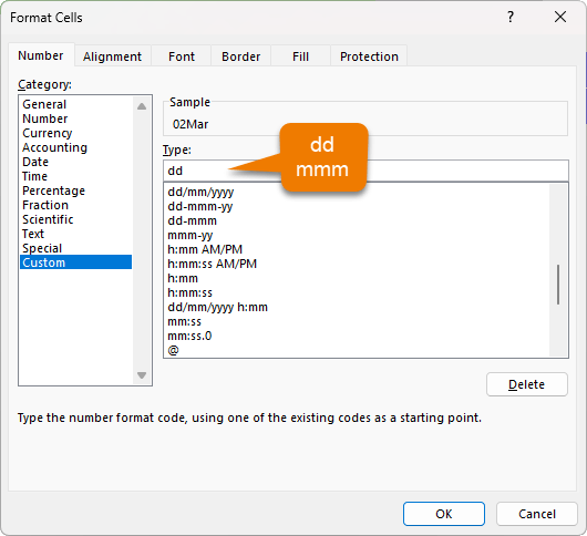
5. Turn on Wrap Text for the cells
This displays the day on one line and the month below it, allowing much narrower columns.
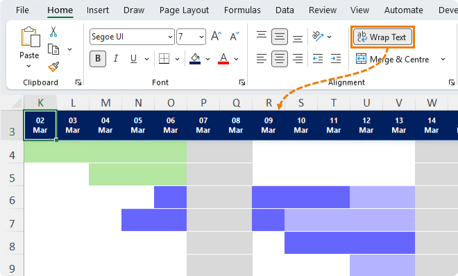
It feels like something Excel should not allow, yet it works perfectly.
Shortcut 3: Alt + Enter
This solves a common structural mistake.
When users want multi-line headers, they often:
- Use multiple rows, which breaks table structure
- Add spaces to force wrapping, which causes issues with sorting and filtering
Instead:
1. Place your cursor where you want the break
2. Press Alt + Enter
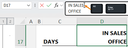
3. Apply Wrap Text format to the cells
This inserts a clean line break within the same cell while preserving proper structure.
Once you start using this, the workarounds stop making sense.
Shortcut 4: F2 (it’s not what you think)
This one removes a very frustrating problem.
When editing formulas inside dialog boxes like Conditional Formatting or Name Manager, arrow keys often select cells instead of moving your cursor.
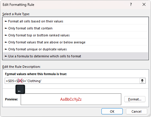
Press F2 first.
This switches Excel into edit mode so arrow keys behave correctly and move within the formula.
Use this anywhere you edit formulas in dialog boxes.
Shortcut 5: Ctrl + Backspace
You scroll away to check something, then lose track of your active cell.
Instead of searching for it, press Ctrl + Backspace.
Excel jumps straight back to your active cell instantly.
Shortcut 6: Tab (this isn’t what you think either)
After selecting a large table, you often end up at the bottom.
If you want to return to the top-left cell of that selection, press Tab.
It instantly repositions you without scrolling.
Tip: You can also press CTRL+Backspace, but that’s two keys when one will also do.
Shortcut 7: Ctrl + .
When working with large selections, navigating between corners can be tedious.
Press Ctrl + . to cycle through each corner of the selected range.
It saves a surprising number of clicks over time.
Shortcut 8: Ctrl + Drag Sheet Tab
Most users duplicate sheets using right-click and menu options.
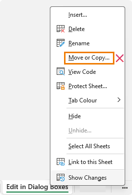
A faster method:
- Hold Ctrl
- Drag the sheet tab
That’s it. The sheet is duplicated instantly.
Once you use this, the menu method feels slow.
Tip: you can also copy sheets to external workbooks using this technique.
Shortcut 9: Ctrl + Click Sheet Navigation Arrows
Large workbooks with many sheets are difficult to navigate.
Instead of scrolling through tabs:
- Ctrl + click the navigation arrows to jump to the first or last sheet
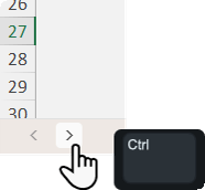
- Or right-click the arrows to display a full list of sheets
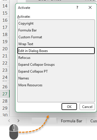
This makes navigating complex workbooks far more efficient.
Shortcut 10: Shift + Scroll
Grouped rows and columns are useful but tedious to manage manually.
Instead:
- Hover your mouse over the cells inside the grouped area, hold Shift and scroll down to collapse
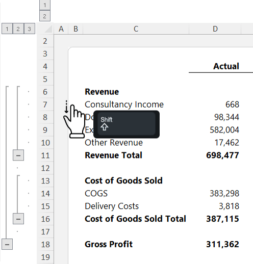
- Hold Shift and scroll up to expand
This works for:
- Grouped rows
- Grouped columns
- PivotTable groups
Tip: Make sure your cursor is inside the worksheet, not over the headers.
Shortcut 11: F3
Named ranges are powerful but easy to forget.
When typing a formula in a dialog box:
- Press F3
Excel displays a list of all named ranges, allowing you to insert them directly.
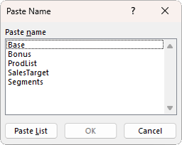
This avoids guessing or switching screens.
Shortcut 12: F4 (not for absolute references)
Most users know F4 for absolute references.
Its more powerful use is repeating your last action.
For example:
- Formatting
- Inserting rows
- Applying borders
Press F4 to repeat the previous step instantly. It’s essentially the same as CTRL+Y, but only one key.
It is one of the simplest ways to speed up repetitive work.
Take Your Excel Skills Further
If you like practical tips like these, you’ll get much more in the Excel Expert course.
It focuses on real-world techniques that improve speed, accuracy, and confidence in Excel.


For the first one, using Ctrl+Shift+U to expand the formula bar… It looked like the gist/intent of the shortcut was that if one had, say, six lines, it would expand all six lines for viewing. But it simply toggles between one line displayed and however many lines I had last expanded it or some other cell. So if that was the regular three lines, it would open it to three lines. If I’d last expanded a cell to 11 lines, it would expand to that. So it was not actually expanding to match the cell contents.
Useful some, so I don’t have to take my hands off the keyboard if I need to view a previously expanded cell, but otherwise… still gotta use the mouse anyway to get it expanded out.
The mechanics of the Ctrl-J shortcut (and of course, Alt-Enter works as well)… When crafting a unique or complicated custom format using such, I often will enter the material that follows the line feed so that I can view it as I type, then the line feed before it pushing it out of view, and finally the beginning. Or rinse and repeat until finished. Of course, if it’s really complicated or new for me, I’ll just write it out in a cell and then copy and paste.
I don’t remember the details of getting the other 8 bit character set (Epson set? The DOS one that gave you lines and such?) but it seems that 30+ years ago, we had a formatting that used those characters to draw boxes as checkboxes or exactly around the cell contents, and so on. ‘Cause any character is a character, and can be used.
Ctrl-Backspace is going to be pretty handy. So is Ctrl-Shift on the navigation tabs. I have one spreadsheet for an idiot we do business with with 200+ sheets rather than one table and some nice slicers and so on for him to view his customers’ activities. There’s a HYPERLINK driven TOC but that doesn’t help when wanting to change formulas across all those sheets. Can’t select them as a group that way… though if someone knows how… so it’s always been a long hard slog. Not now though!
For #12, I’d say it could be helpful to people to mention that Ctrl-Y and F4 have an aspect to their “Repeat…” action that most are not cognizant of: They repeat that last action wherever they selection currently is, as long as it makes sense. What’s the difference? ‘Cause that sounds a lot like “Repeat…” right?
We tend to think of Ctrl-Y, for instance, as the opposite of Ctrl-Z… and it is, if used in that fashion. But say you format cell A3 with a red font and want to format another cell, perhaps D3 or F23:H31 with the same red font. Select the cell or cells and press Ctrl-Y or F4 and it will not undo some Undo, but rather perform that same formatting you just did to A3. And all your selected cells will have the same red font. Perhaps you’re doiing the Paste|Special|Multiply (by 1) trick to change or force a change of some cells formatted as text to cells formatted as number. Do it, with all the keystrokes or mousing, then select any other range you also need done and press Ctrl-Y or F4 and do the same with a single keystroke.
A small difference, but isn’t so much of usefulness in Excel a matter of finding small things that almost certainly were not intended for your need and using them to do it anyway? Kinda quintessential Excel, really. The fun part anyway.
Thanks for sharing your insights, Roy! Correct, CTRL+SHIFT+U expands the formula bar to the last size. It would be nice if it recognised the rows the formula occupied and expanded accordingly, but alas it doesn’t. I still use it all the time despite this shortcoming.
Nice! I would add something very helpful for me: Alt+; to select only visible cells (instead of F5/Ctrl+G -> and then clicking Special and visible only)
Nice! Thanks for sharing, Tomek.
Thank you tomek! That solves a problem I often have with one spreadsheet.