Excel Data Analysis Without Formulas

Do you spend hours every month building Excel reports full of repetitive formulas? You're not alone. Many professionals use hundreds of SUMIFS, COUNTIFS, and AVERAGEIFS formulas across multiple sheets just to answer a handful of business questions.

But what if there was a smarter, faster way?

In this post, you'll learn how to replace countless formulas with a single dynamic PivotTable. Not only will this technique save you time, but it will also make your reports easier to update, especially when last-minute changes come in (as they always do!).

Watch the Data Analysis without Formulas Video

Get the Dataset and Example File

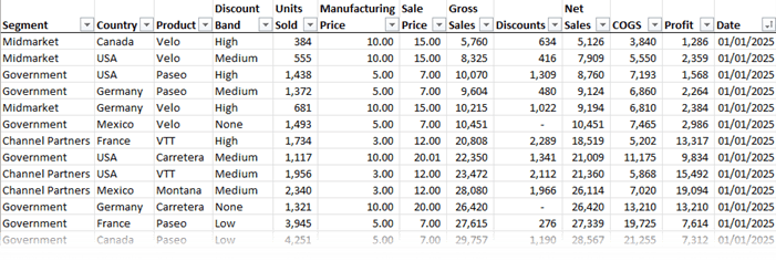
The Dataset We’ll Use

Here’s what our example dataset includes:

• Categorical columns: Segment, Country, Product, Discount Band
• Numeric columns: Units Sold, Net Sales, Profit, etc.
• Date column: So we can group by months or years

This is the kind of data most businesses track and it’s perfect for PivotTables:

Reporting Requirements

Let’s say your manager drops by at 4pm on a Friday asking for the following summary:

1. Units sold by Product
2. Net Sales by Product
3. Profit by Segment
4. Average Profit per Unit by Product & Segment
5. Percentage Profit Margin by Segment

Instead of jumping into a spreadsheet jungle of formulas, here’s the faster, smarter way using PivotTables.

Step-by-Step: Create a Dynamic Report with One PivotTable

1. Format the Data as a Table

Use Ctrl + T to convert your dataset into an Excel Table.
Why? It ensures your PivotTable automatically expands when new data is added.

2. Insert a PivotTable

Go to Insert tab > PivotTable, then for the first 3 measures:

Units Sold by Product

• Rows: Product
• Values: Units Sold

Add Net Sales

• Still in the same PivotTable, add:
  • Values: Net Sales

Profit by Segment

• Rows: Segment
• Values: Profit

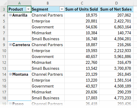
Tip: You can collapse or expand row groups to drill into or hide details easily – right click the Product or Segment fields > Expand/Collapse.

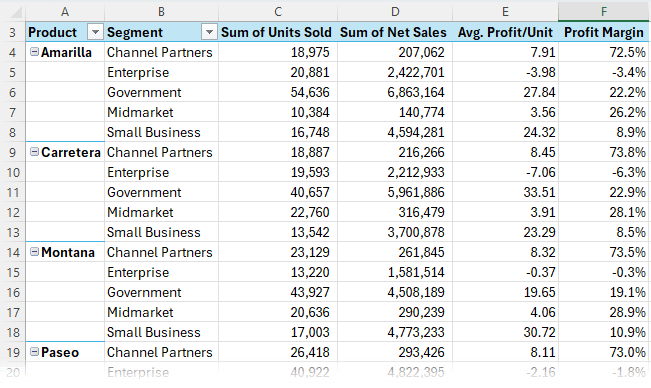
3. Add Calculated Fields

The last two measures require Calculated Fields. To add custom calculations, go to:

PivotTable Analyse tab > Fields, Items & Sets > Calculated Field

Average Profit per Unit

• Name: Avg. Profit/Unit
• Formula: =Profit/'Units Sold'
• Format: 2 decimal places

Profit Margin (%)

• Name: Profit Margin
• Formula: =Profit/'Net Sales'
• Format: Percentage, 1 decimal place

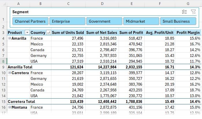
Instant Updates with PivotTables

Once your PivotTable is set up:

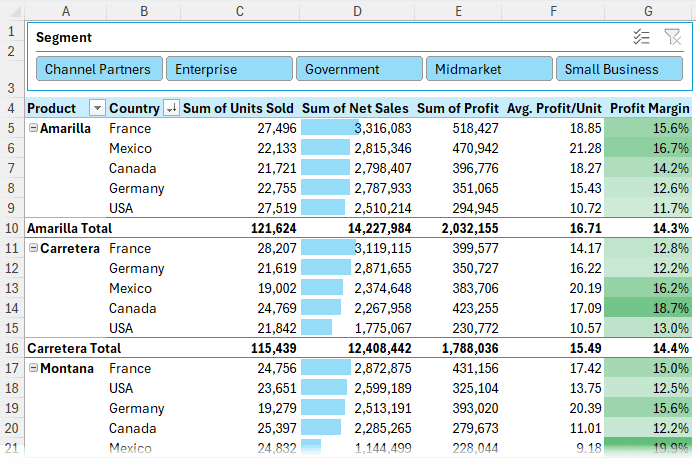
• Want to show the data by Country instead of Segment? Just drag and drop – remove Segment and replace it with Country.
• Want to add interactivity? Right click the Segment field > Add as Slicer:
  • Format it with 5 columns and position above the PivotTable for easy access.
  • Match the style to your PivotTable

Add Conditional Formatting

Help your manager quickly spot trends:

• Profit Margin → Use Color Scales (e.g., green for high values, white for low)
• Net Sales → Use Data Bars, set the color to match your PivotTable style
• Sort Net Sales in descending order for clear ranking

Updating the Report is Easy

Next month, when new data arrives:

1. Add it to the bottom of the Excel Table source data
2. Click Refresh (Data tab or right-click PivotTable) and your report updates instantly!

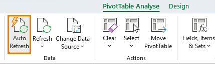
Excel 365 Users: Try Auto-Refresh

If you're using Microsoft 365, enable Auto-Refresh (currently in beta) to automatically update your PivotTable when the source data changes.

Results: A Dynamic Report with Zero Formulas

With just one PivotTable and a few calculated fields, you've built:

• A reusable, filterable report
• That’s easy to update
• With zero formulas
• In record time

You’re done - and it’s not even 5pm yet!

Ready to Take It Further?

PivotTables are amazing, making light work of reports and enabling you to glean insights in minutes. Get up to speed with them fast in our PivotTable Quick Start course.

Summary

Task	Traditional Method	PivotTable Method
Summarise data	Formulas (SUMIFS, etc.)	Drag-and-drop
Add custom calculations	More formulas	Calculated Fields
Update report with new data	Adjust formulas, ranges	Click Refresh
Last-minute layout changes	Rebuild formulas/sheets	Drag to rearrange
Filter by category (e.g. Segment)	Add filter rows manually	Use Slicers
Highlight key metrics	Conditional formatting setup	Works seamlessly