
Some Excel functions have exciting names like XLOOKUP, FILTER, and LET. Others sound like they belong in a maths textbook.
Functions like ABS, SIGN, REPT, TRUNC, and CELL don't get much attention, but each one solves a surprisingly common problem. Better still, they're available in virtually every version of Excel, so you don't need Microsoft 365 to use them.
Let's look at five underrated Excel functions that can make your formulas smarter, your reports easier to read, and your spreadsheets more reliable.
Table of Contents
Watch the Video

Get the Example File
Enter your email address below to download the free file.

1. ABS: Ignore the Sign and Focus on the Size
What Does ABS Do?
The ABS function returns the absolute value of a number by removing its plus or minus sign.
=ABS(number)
For example:
=ABS(-10)
returns:
10
On its own, that might not seem very exciting. But used in the right situation, ABS can prevent some seriously misleading calculations.
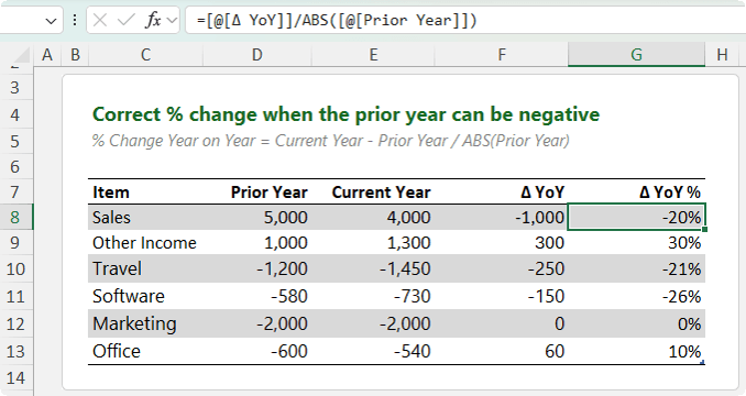
Example 1: Calculating Year-on-Year Percentage Change
A common formula for calculating percentage change is:
=(Current Year-Prior Year)/Prior Year
This works perfectly for revenue figures that are always positive.
The problem comes when the prior-year figure is negative, such as expenses or losses.
Suppose travel costs increased from -$1,200 to -$1,450.
The dollar change is:
-250
If you divide by the negative prior-year amount, Excel returns a positive percentage, suggesting performance improved when, in reality, costs increased.
The solution is to make the denominator positive:
=(Current Year-Prior Year)/ABS(Prior Year)
Now the percentage correctly reflects whether the change was favourable or adverse:
Example 2: Checking Invoice Tolerances
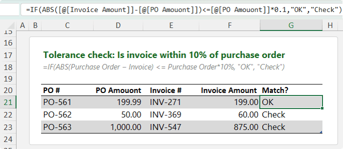
Imagine a business allows supplier invoices to vary by up to 10% from the purchase order amount.
You don't care whether the invoice is higher or lower. You only care about the size of the difference.
ABS makes this simple:
=IF(
ABS(InvoiceAmount-POAmount)<=POAmount*0.1,
"OK",
"Check"
)
Instead of testing for both positive and negative variances, ABS converts everything into a positive number so you only need one test:
2. SIGN: The Secret to OR Logic in SUMPRODUCT
What Does SIGN Do?
The SIGN function returns only three possible results:
=SIGN(number)
- Positive numbers return 1
- Negative numbers return -1
- Zero returns 0
At first glance, it doesn't seem particularly useful. But it becomes incredibly powerful when building logical tests.
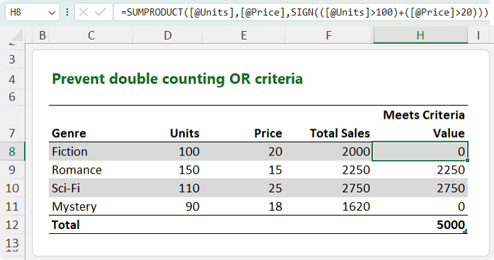
Example: Avoiding Double Counting with SUMPRODUCT
Suppose you want to calculate total sales for books that:
- Sold more than 100 units, OR
- Cost more than $20.
A common approach is:
=(Units>100)+(Price>20)
Because Excel treats TRUE as 1 and FALSE as 0, adding the tests together works well until both conditions are TRUE.
In that case:
1 + 1 = 2
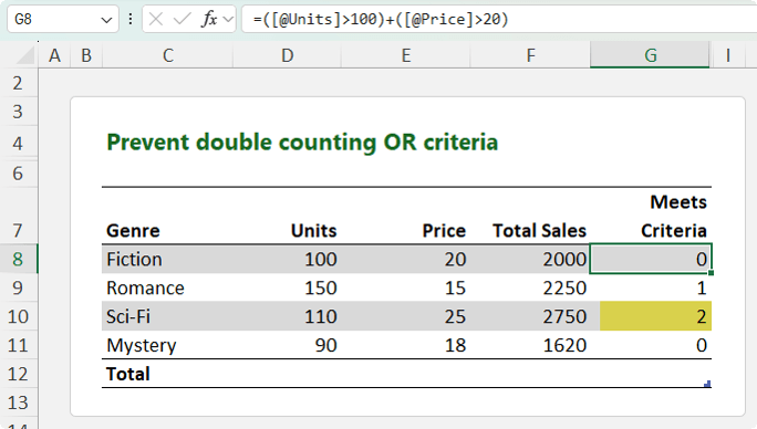
When used inside SUMPRODUCT, those rows get counted twice.
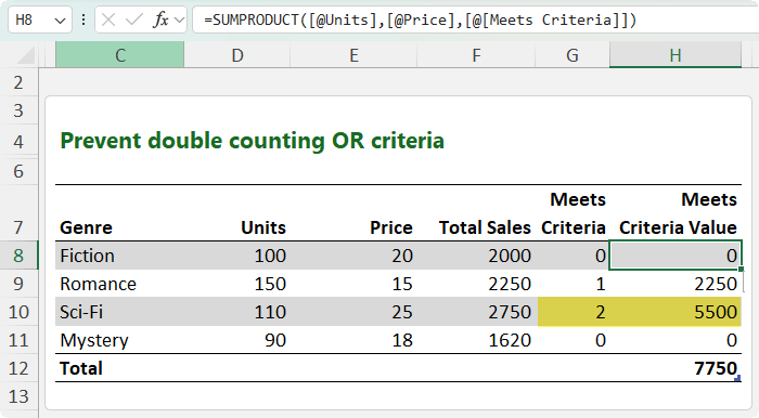
SIGN fixes the problem:
=SIGN((Units>100)+(Price>20))
The result:
- 0 stays 0
- 1 stays 1
- 2 becomes 1
Every qualifying row is included once and only once.
This is a brilliant technique whenever you're creating OR logic with SUMPRODUCT.
3. REPT: Create Charts Inside Cells
What Does REPT Do?
The REPT function repeats text a specified number of times.
=REPT(text, number_of_times)
For example:
=REPT("●",5)
returns:
●●●●●
Simple, but surprisingly powerful.
Example: Build Mini Charts in Cells
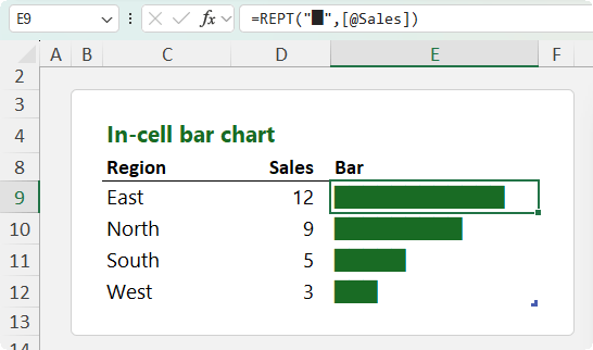
Suppose you have sales figures by region.
Instead of inserting a chart, you can create a visual directly inside the worksheet:
=REPT("█",Sales)
The result is an in-cell bar chart that grows and shrinks with your data.
These mini charts are great for:
- Dashboards
- KPI reports
- Heat maps
- Scorecards
- Executive summaries
You aren't limited to block characters either. Stars, circles, and shaded symbols all work well.
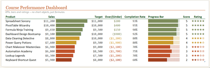
Click here for the full REPT function tutorial and learn how to build the dashboard above.
REPT is one of those functions that can make a report feel far more interactive without using a single chart object.
4. TRUNC: Remove Decimals Without Rounding
What Does TRUNC Do?
The TRUNC function removes decimal places without rounding.
=TRUNC(number)
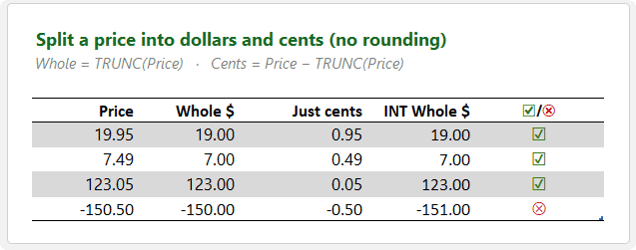
Example 1: Split Dollars and Cents
Given a price of:
$19.95
The formula:
=TRUNC(19.95)
returns:
19
The cents can then be calculated as:
=Price-TRUNC(Price)
which returns:
0.95
TRUNC vs INT
For positive numbers, TRUNC and INT return the same result.
The difference appears with negative values.
Consider:
-150.50
TRUNC returns:
-150
INT returns:
-151
This is because:
- INT always rounds down.
- TRUNC removes decimals and moves toward zero.
When negative numbers are possible, this distinction becomes very important.
Example 2: Calculate Whole Items You Can Afford
Suppose you have:
- Budget: $500
- Licence cost: $79
The calculation:
=500/79
returns:
6.33
But you can't buy one-third of a licence.
TRUNC gives you the number of whole licences:
=TRUNC(500/79)
which returns:
6
To calculate the money left over:
=500-TRUNC(500/79)*79
Or even better:
=MOD(500,79)
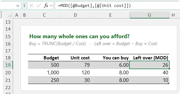
This same pattern works for:
- Boxes in a shipment
- Full teams from a group of people
- Whole weeks in a project
- Equipment allocation
- Resource planning
5. CELL: Ask Questions About Your Worksheet
What Does CELL Do?
Unlike most functions, CELL doesn't perform calculations.
Instead, it returns information about a cell.
The syntax is:
=CELL(info_type, reference)
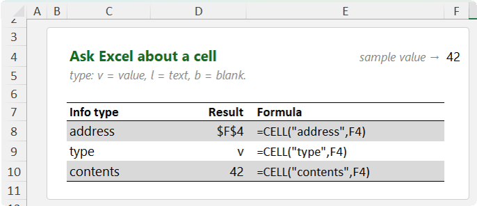
For example:
=CELL("address",F4)
returns:
$F$4
You can also ask:
=CELL("type",F4)
which returns:
- v for value
- l for text label
- b for blank
Or:
=CELL("contents",F4)
which returns the cell's contents.
Example: Display the Current Worksheet Name Automatically
One of the most practical uses of CELL is creating dynamic worksheet titles.
The formula:
=MID(
CELL("filename",A1),
FIND("]",CELL("filename",A1))+1,
31
)
extracts the current sheet name from the workbook's full file path.
This is incredibly useful for:
- Monthly reports
- Dashboard tabs
- Duplicated worksheets
- Templates
Rename the sheet and the title updates automatically.
One thing to remember: the workbook must be saved first. Until the file has a name, CELL("filename") has nothing to return.
Final Thoughts and Next Steps
None of these functions are particularly impressive on their own.
The magic happens when you know when to use them and how to combine them.
- ABS fixes misleading percentage calculations.
- SIGN prevents double counting in OR logic.
- REPT creates simple but effective visualisations.
- TRUNC helps you work with whole quantities.
- CELL adds dynamic information to your reports.
This is the real power of Excel. It isn't about knowing one giant formula. It's about having lots of small techniques you can combine to solve problems elegantly.
Want to get better at writing formulas like these? My Advanced Excel Formulas course will help you stop guessing and start building clean, confident formulas you can trust.



Another, IMHO, immensely powerful use for =CELL(“filename”,A1) is to return the path of the file. Employed as a power query parameter, it enables you to package files and data folders together in a zip file that means, once extracted AND saved; when the queries are refreshed, they will automatically pick up their dependent file/data location absolute path/s. Logic can be added to discriminate and accommodate local, OneDrive, SharePoint, etc.. save locations.
Yes, great use case, Dave. Thanks for sharing. I also cover this in my Power Query course.