13 Time-Saving Excel Productivity Tricks

Think you know Excel? Think again. These 13 hidden gems will streamline your work, eliminate frustration, and unlock features most users don’t even know exist—no matter your level of experience. Best of all, you can try them yourself using the downloadable file linked to below.

Watch the Video

Get the Practice File

1. Copy Only Visible Cells

Ever copied a filtered list and ended up with hidden data sneaking in? That’s because Excel copies everything, hidden or not.

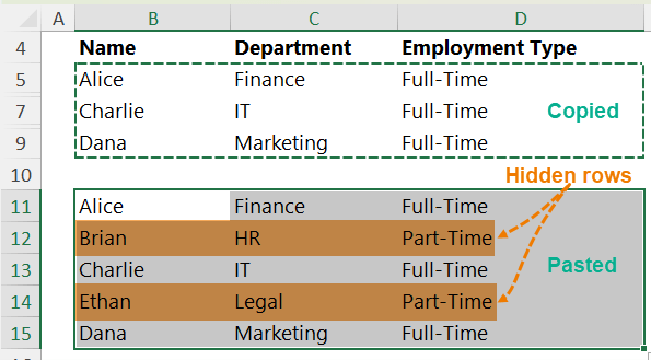
Here’s the fix:

• Select your range
• Press Alt + ; (semicolon) to select only visible cells

• Paste as usual

Now, no hidden surprises—just the data you want.

2. Live Snapshots

Want a live snapshot of one sheet on another? A Linked Picture gives you exactly that.

1. Copy your range (Ctrl + C)
2. On another sheet where you want the snapshot: Home tab → Paste → Linked Picture

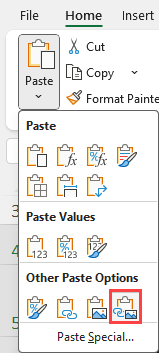
It floats above the grid and updates in real time—like a live security feed for your spreadsheet. You’ll notice images don’t render as well in the linked picture, but text is quite clear:

Earlier Versions of Excel - Camera Tool: if you don’t have a version of Excel with the Linked Picture option, you can use the Camera Tool. You’ll need to add it to your Quick Access Toolbar. To do this:

1. Right-click the quick access toolbar > customise Quick Access Toolbar…
2. Select All Commands from the ‘Choose commands from’ drop down.
3. Locate the Camera tool in the list and click ‘Add’

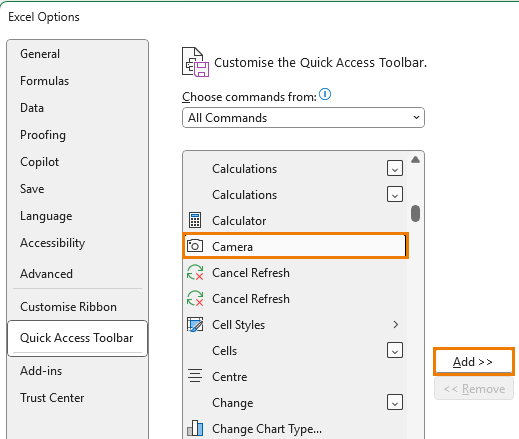
You can now select the range of data you want a live snapshot of and click the Camera tool to take a copy. Click again to create the linked picture object on the sheet you want.

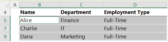
3. Remove Duplicates vs Unique Lists

You probably know about Data → Remove Duplicates. But here’s an option if you want to retain the original data:

• Create a non-destructive unique list:
  1. Select the data including the heading
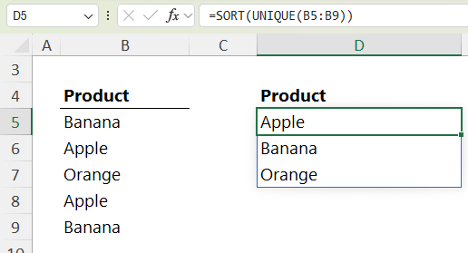
  2. Data tab → Advanced

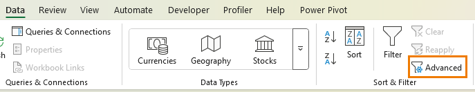
• Choose “Copy to another location”
• Tick “Unique records only”

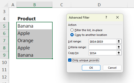
Or make it dynamic and sorted:

=SORT(UNIQUE(B5:B7))

Now the list updates automatically when your data changes.

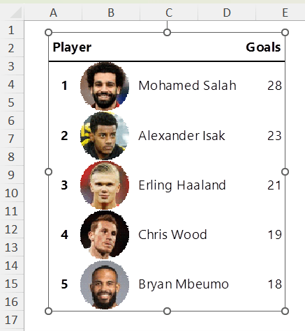
4. Build a Bar Chart In a Cell

Create a mini bar chart using a formula:

=REPT("|",C5)

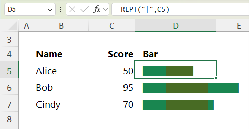
• Use the Playbill font for best results
• Change font colour to match your theme
• Updates as values change

Simple. Visual. Effective.

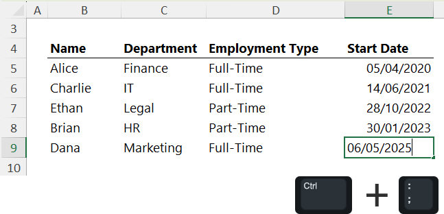
5. Insert Today’s Date Instantly

Typing today’s date manually? Don’t.

• Just press Ctrl + ; (semicolon) followed by Enter.

6. Debug Formulas Like a Pro

Formula not working? Try this:

• Select part of the formula while editing
• Excel shows the result as a tooltip (in newer versions)

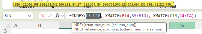
• Or press F9 to evaluate manually
• Ctrl + Z or Escape to undo changes

Once you get a taste for decoding formulas like this, you’ll want to level up fast.

I’ve got a full course here on Advanced Excel formulas that teaches you how to create error-proof, dynamic spreadsheets.

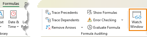
7. Use the Watch Window

Tracking values across multiple sheets? The Watch Window makes it easy:

• Formulas → Watch Window

• In the dialog box, Add Watch
• Add any cells you want to monitor

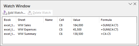
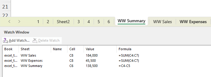
It floats wherever you want—track totals, KPIs, or key dates without jumping between sheets.

Pro tip: drag slowly to the bottom/side of the Excel window, or above the formula bar to dock it in place.

8. Move Rows and Columns Without Cut-Paste

Need to rearrange a row or column?

• Select the row/column, hover the edge until you see the 4-sided arrow

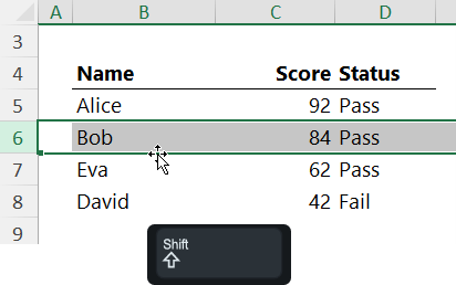
• Hold Shift, drag, and drop

Excel slides everything perfectly into place. Bonus: Hold Ctrl + Shift to copy instead of move.

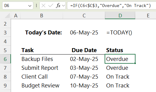
9. Auto-Update Dates with TODAY

Use =TODAY() to always show the current date, pulled from your PC clock.

Example:

=IF(C6<$C$3,"Overdue","On Track")

This compares a due date in cell C6 to today’s date in cell C3 and labels it accordingly:

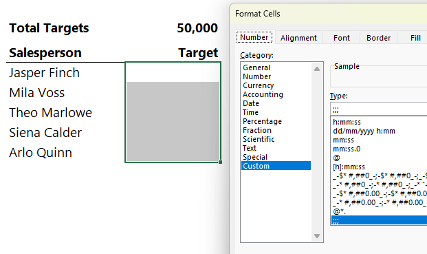
10. Hide Values With 3 Semicolons

Don’t want data visible, but still need it in the sheet?

• Select cells > press Ctrl + 1 → Number → Custom
• Enter ;;;

Data disappears from the cell face:

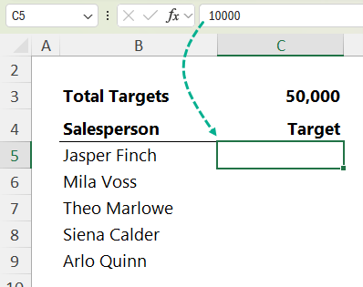
But still works in formulas:

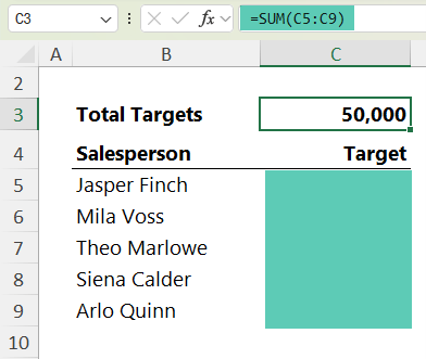
And shows in the formula bar:

11. Fix Broken Percentage Formatting

Formatted a number as a percentage and got 2500% instead of 25%?

Here’s the fix:

1. Type 100 in an empty cell → Ctrl + C
2. Select the incorrect percentages
3. Paste Special → Divide

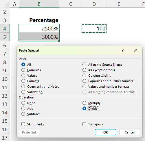
Now they’re accurate and correctly reflect the formatting.

12. Use Custom AutoFill Lists

You can go beyond days and months:

• File → Options → Advanced → Edit Custom Lists

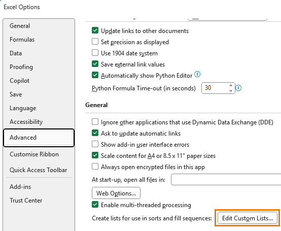
• Type or import your list (e.g. department names)

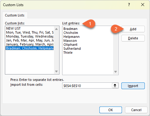
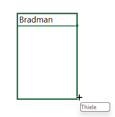
• Once saved, just type the first item and drag to auto-fill the rest

Great for repetitive entry with zero typos.

13. Repeat Table Headers When Printing

Avoid the classic “What’s this column?” problem on page 2 of printouts.

• Page Layout → Print Titles

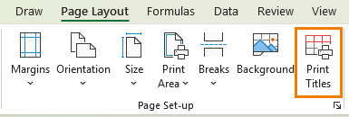
• On the Sheet tab, under "Rows to repeat at top", select your header row

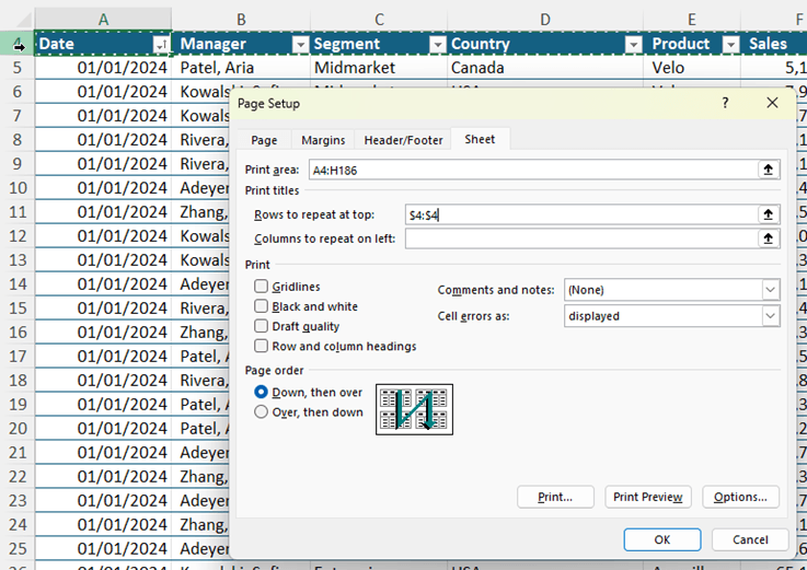
• Optional: Select columns to repeat on the left

Now every printed page includes headers for clarity.

Bonus: The One Excel Trick I Use Every Day

If I had to pick one Excel trick I rely on daily, this would be it. Once you discover it, there’s no going back.

👉 Watch the video here

Twelve minutes that could change how you use Excel—for years to come.