Custom number formats are one of the most overlooked features in Excel. They change how numbers look in a cell while keeping the underlying value intact. That means your formulas, PivotTables, and charts continue to work exactly as expected.
In this guide, you’ll learn 10 practical custom number format examples you can start using immediately to make your reports cleaner, faster to read, and more professional.
Table of Contents
- Watch the Excel Custom Number Formatting Video
- Get the Example Workbook & Cheatsheet
- What Are Excel Custom Number Formats?
- 1. Scale Numbers to Thousands or Millions
- 2. Add Colors Without Conditional Formatting
- 3. Display Text Based on Values
- 4. Hide Zero Values
- 5. Add Symbols Like Arrows or Icons
- 6. Format Phone Numbers Automatically
- 7. Create Custom Date Formats
- 8. Add Units Like km or kg
- 9. Hide Cell Values Without Deleting Them
- 10. Add Leading or Trailing Characters
- Why Custom Number Formats Matter
- Get the Full Guide
Watch the Excel Custom Number Formatting Video

Get the Example Workbook & Cheatsheet
Enter your email address below to download the free file.

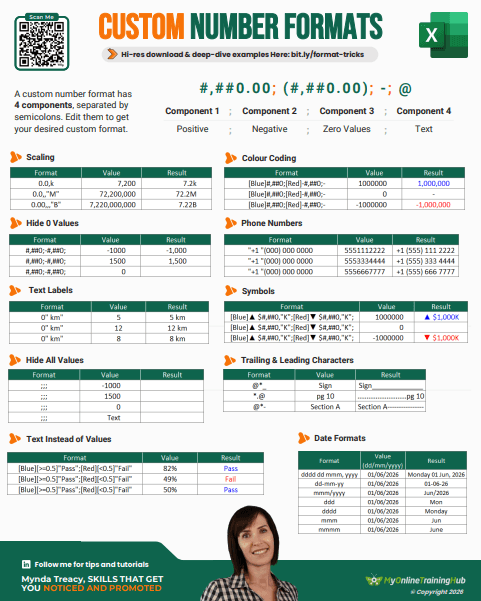
What Are Excel Custom Number Formats?
Custom number formats are codes that control how values appear without changing the data itself. Instead of rewriting formulas or adding helper columns, you can apply a format that improves readability and presentation instantly.
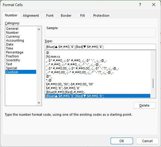
You can access them with Ctrl + 1, then go to the Custom category.
They consist of 4 sections, each separated by a semicolon:
Positive ; Negative ; Zero ; Text
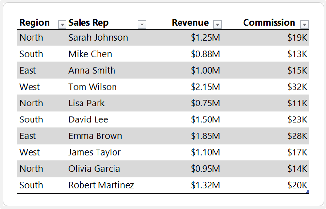
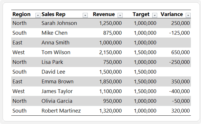
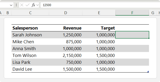
1. Scale Numbers to Thousands or Millions
Large numbers are hard to read and compare. Instead of showing 1,250,000, you can display it as 1.25M.
Use this format:
#,##0.00,,"M";-#,##0.00,,"M"
Each comma removes three zeros from the display. Two commas convert values to millions.
For thousands:
#,##0.00,"K";-#,##0.00,"K"
Tip: Keep your scale consistent across the report and move the unit into the column header instead of formatting every number to reduce clutter when working with large tables.
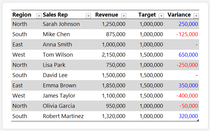
2. Add Colors Without Conditional Formatting
You can apply colour directly inside a number format.
Example:
[Blue]#,##0;[Red]-#,##0;-
This format:
- Displays positive numbers in blue
- Displays negative numbers in red
- Replaces zeros with a dash
This is faster than setting up conditional formatting and keeps your workbook lighter.
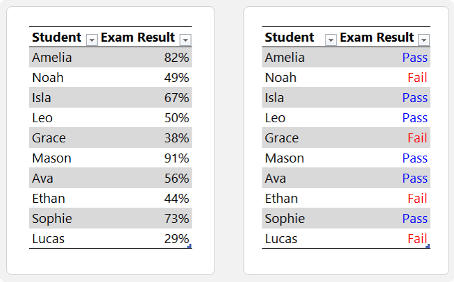
3. Display Text Based on Values
You can replace numbers with text such as Pass or Fail.
Example:
[Blue][>=0.5]"Pass";[Red][<0.5]"Fail"
This allows you to:
- Keep numeric values for calculations
- Display clear labels for users
- Avoid extra IF formulas
4. Hide Zero Values
Zeros can clutter reports and distract from meaningful data.
Use:
#,##0;-#,##0;
The empty third section hides zeros while keeping them available for calculations.
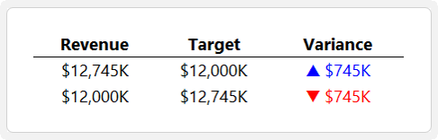
5. Add Symbols Like Arrows or Icons
Symbols can make reports easier to interpret at a glance.
Example:
[Blue]▲ $#,##0,"K";[Red]▼ $#,##0,"K";
Use symbols like:
- ▲ for positive
- ▼ for negative
You’ll find symbols on the Insert tab:
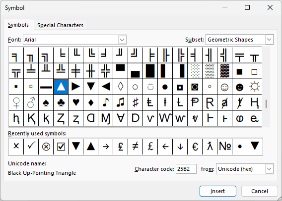
Tip: You can also use checkmarks and crosses from fonts like Wingdings.
6. Format Phone Numbers Automatically
Instead of typing spaces or apostrophes, use a format.
Example:
"+1 "(000) 000 0000
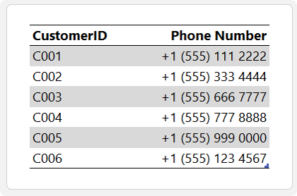
This ensures:
- Consistent formatting
- Proper handling of leading zeros
- Faster data entry
7. Create Custom Date Formats
Default date formats are limited. Custom formats give you full control.
Examples:
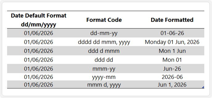
You can tailor dates for:
- Reports
- Dashboards
- Regional preferences
The underlying value remains a true Excel date, so grouping and calculations still work.
8. Add Units Like km or kg
Avoid converting numbers to text just to add units.
Use:
0" km"
This keeps values numeric while making them easier to read.
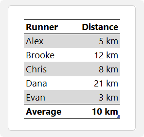
Tip: For large datasets, add units in the column header instead of every cell.
9. Hide Cell Values Without Deleting Them
If you need to hide values temporarily:
;;;
This hides:
- Positive values
- Negative values
- Zeros
- Text
The data is still visible in the formula bar and usable in formulas:
Important: This is not a security feature.
10. Add Leading or Trailing Characters
You can create dynamic visual effects for forms or layouts.
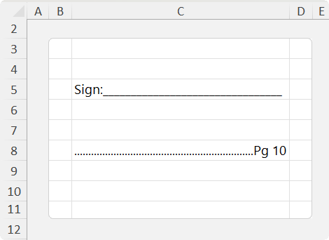
Example for signature lines:
@*_
This repeats the underscore to fill the cell width.
Example for dotted leaders:
*.@
This creates leading dots before text, useful for tables of contents.
Why Custom Number Formats Matter
These small formatting changes can dramatically improve how your reports are understood. You can:
- Reduce visual clutter
- Improve readability
- Avoid unnecessary formulas
- Keep your data fully functional
Once you start using them, they quickly become part of your everyday workflow.
Get the Full Guide
If you want to go further, check out my comprehensive custom number format guide that goes into more detail on literal characters, special characters, digit placeholders and more.

