PivotTables are a treasure trove of features and one that has been brought out of the dungeons in more recent Excel versions is ‘Show Values As’.
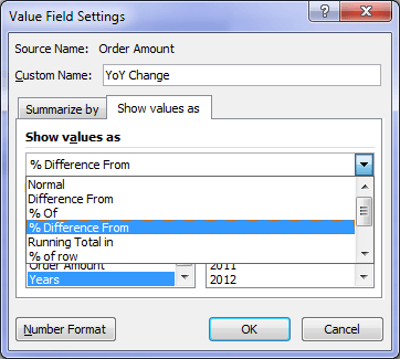
In Excel 2007 it was hidden 3 clicks away in the Value Field Settings dialog box (see below):
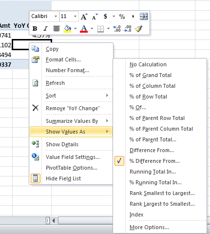
Then in Excel 2010 it was given prime position in the right-click Context Menu, and rightly so:
In Excel 2010 there are also some new functions like Rank and % Running Total In to name a couple.
In this tutorial I’m going to show you how to calculate Year on Year variances, both absolute values using Show Values as > Difference From:

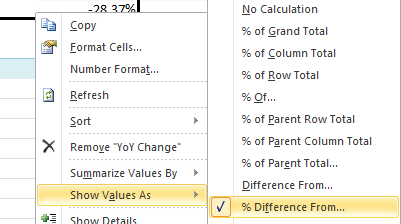
And as a percentage using Show Values As >% Difference From:
Enter your email address below to download the sample workbook.
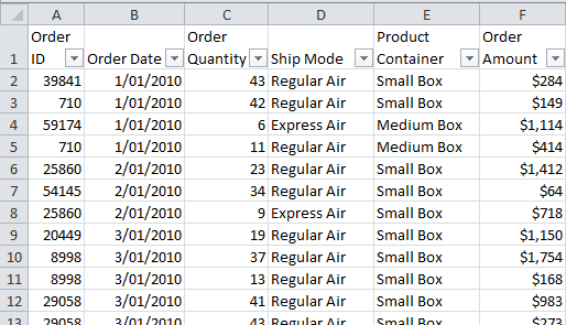
Here is a sample of my data:
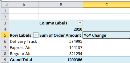
Here is my PivotTable with Order Amount summarised by Ship Mode and Year:
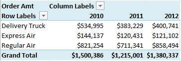
Now I want to add columns for the year on year change (YoY Change).
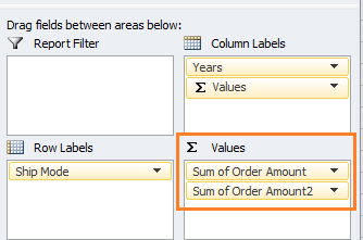
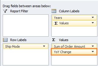
Step 1: Drag another instance of the Order Amount field to the Values area in the field list, so now you have it there twice:
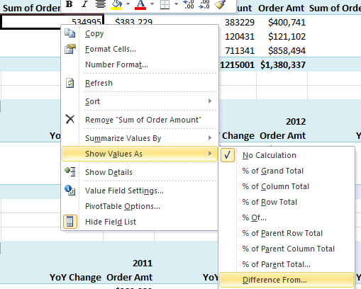
Step 2: In the PivotTable right-click any of the cells containing the second Sum of Order Amount > Show Values as > Difference From:
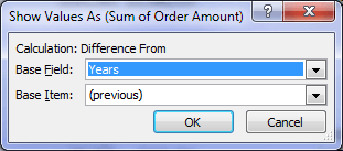
Step 3: Choose Years as the Base Field and Previous as the Base Item in the dialog box that pops up:
Step 4: Next we can rename the Column Labels so they’re more meaningful. To do this just type straight in one of the cells containing the column label you want to change, like I’ve done in cell C5 below (Tip: the name must not be the same as any of the source data column headers):
This will update all of the column labels and the name in the field list:
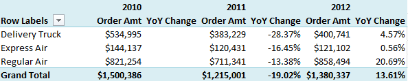
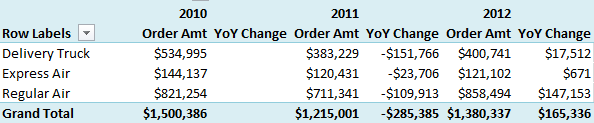
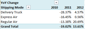
Voila, your PivotTable now shows the year on year change in Order Amounts by Shipping Mode:
Year on Year Percentage Change
We can also show values as % Difference From. The steps are the same except in step 2 you choose % Difference From:
Tip: You don’t need to have the Order Amount column in your PivotTable to display the YoY Change:
Since the YoY Change is not calculated using the actual values you see in the PivotTable, it is calculating using the source data.
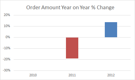
Which means you could plot just the Year on Year Change in a PivotChart if you wanted.

In your example, how could a CAGR column (annualized growth rate from 2010 to 2012, = (‘2012’/’2010’)^(1/2)-1) of data and have that data be formatted as a percentage even while the sales data stays formatted as currency?
Hi Casey,
Please post your question on our Excel forum where you can also upload a sample file that shows the format and layout of your data and we can help you further.
Mynda
Is there a way to filter within the pivot table by the % difference from rather than the sum of the base value? I am using Excel 2019.
I am trying to show a Y/Y or Q/Q Top 10 and Bottom 10 % changes in revenue from a list of hundreds of locations. I’d like the time period to be controlled by a slicer or timeline.
Please help!
thanks
Hi Steve, Yes, select the row/column label you want the top two displayed for > click on the filter button > value filters. If you get stuck, please post your sample Excel file and question on our forum where we can help you further.
I found this page trying to create a chart like the last image in your article, which chart did you use?
Hi CT,
It’s a column chart.
Cheers,
Catalin
Hi Mynda,
I have a pivot table problem with top 20 customer and year on year sales. I’m looking to have the current top 20 customer in the current year and have these customer sales figures for prior year and prior year+1. As you know when you have the top 20 customer sales the pivot table works out the top customer over the grand total sales. How can I do a work around to ignore the grand total?
Hi Barry,
You can’t, sorry. If you have all of the years in the PivotTable then the filter for top N will be taking all of the years into consideration. There’s no way to tell it to filter on a single year unless you filter for that year.
Mynda
This is late but a solution. If you can add columns to the base data, add two. In the first one use the countifs and sumifs functions to add all the sales for a customer in the customers first row. Then use the countifs and rank functions to list the customers ranks.
Example for row 2500 and customer name in column A and sales amount in column B. This sumifs formulas are in column C and rank formulas are in D, year is in column E
Sumifs: =if(countifs($A$1:$A2500, A2500)=1,sumifs($B:$B,$A:$A,A2500,$E:$E=2020),0)
Rank: =if(countifs($A$1:$A2500,A2500)=1,rank(C2500,$C:$C,0),index($D:$D,match(A2500,$A:$A,0))
Make column D the first column in your pivot table and filtered on it.
Thanks for sharing, Patrick!
Hi,
I have a pivot table showing the % difference in sales from 2016 to 2017 by customer. It works well except for those customers who had no sales in 2016. The % difference field shows a 0% change even though there are 2017 sales showing. Is there some setting I’ve overlooked that will generate a % difference value if 2016 sales don’t exist? I’ve played around with the PivotTable option “For empty cells show”, but it doesn’t matter if a 0 is entered or not –there is no % change generated.
Hi Seth,
This is mathematically correct. A percentage change requires a starting value for 2016 other than zero. You cannot calculate a percentage change if 2016 had no sales.
Mynda
Hi Mynda,
My question goes into the same direction. I need to have a table that compares % changes from year to year, e.g. 2020 vs 2019. If a customer has no sales in 2019 the field should say “New” and if there are no sales in 2020 it should say “Lost”. I understand that this fantastic pivot function “show difference in %” can only be used if there are values for both years but maybe you have an idea how I could do that.
I was thinking of having a formula for the “New/Lost” bit already in the base data, then having the pivot for the % changes for customers having sales in both years and then somehow using a static table combining both.
However, it all seems very cumbersome to me, maybe you can point me in the right direction? I can provide sample data/table if needed.
Appreciating your help!
Mirjam
Hi Mirjam,
The PivotTable won’t return a text value of ‘new’ or ‘lost’ in place of a numeric result, so this type of solution would need to be built outside of the PivotTable. If you get stuck or need some pointers, please post your question and sample Excel file on our forum where we can help you further.
Mynda
Hi,
I am using a PowerPivot sourced pivot table. When I follow the steps below I get an #NA error in the % Difference field. Any idea what is going on? I’ve tried it with all years or just 2 years selected and tried with years in the column field and without.
Hi Steve,
Not sure. It should work the same with Power Pivot. I tested it just now and got the same results with both an implicit measure and explicit measure. You can post your file and question on our Excel forum and we’ll take a look.
Mynda
Hello,
I’m trying do do something very similar to this and it works great. However, when I try to sort by the new year over year difference column it does not show the difference in the ascending order as I would like.
Is there a way to sort on a “Difference from” column?
Hi Jay,
No, unfortunately the sort won’t work on columns that use reference points to calculate.
Mynda
Welcome to Mynda
You are unparalleled. Thank You for sharing your knowledge and skills.
Just having a senior moment …
Can you please show how you went from the year-on-year pivot table to the chart at the bottom?
Hi George,
In the Excel file available for download in the blog post above you’ll see the PivotTable feeding the chart is slightly different to the PivotTable above it. Here is the link to download the workbook to save you looking for it.
Mynda
Great! Found this my self, but i am stucked at the problem two (2) problems.
a) Removing the first year.
In your example 2010. If you like it not to show that, as it doesn’t add any information.
b) Dynamic base year
You are using “previous”, if you use a base year, like 2010, in how is every thing going from 2010 (my electricity bill in my case 🙂 Have you find a solution for having a dynamic base line year? Preferably from a “Excel slicer”?
Hi Carl,
I agree it’s annoying having 2010 display when there is no YoY change value for that year, but the PivotTable has to start somewhere and it cannot calculate a change if the year is not present in the PivotTable. In other words, if you remove/filter ut 2010 then you get a blank YoY change for 2011.
So, the best option is to simply hide the column for the first year, or at least the YoY change column that contains blanks.
Mynda
Thanks for your posts.
I was driving myself crazy today trying to find a good way to present year over year analysis without over-complicating the chart. This is a perfect solution. My only issue is the negative growth crosses over the axis names, so I need to decide if it the title look better at the top or bottom on the chart.
Glad we could help, Mary Beth.
I want to calculate amounts year over year in absolute value not in percentage, how can I do. Is there any tool to get it?
Thanks.
Hi Bertha,
Please take a closer look at the tutorial, you have both versions there, to display absolute values (Show Values as > Difference From:) or percentages (Show Values as > % Difference From:).
Catalin
Hi Mynda,
Thanks. I have a very basic question – how did you get the ‘Years’ column to appear in the pivot table, though it is not present in the raw data set.. I got the rest of the tutorial. 🙂
Thanks,
Adi
Hi Adi,
I grouped the dates into years. You can read more about how to group data in PivotTables here.
Kind regards,
Mynda
Thanks Mynda,
I tried that, and could group it into years. However the difference I noted was that your Pivot Table Field List explicitly has a field “Years”, while mine does not. Sorry to bother you with this question – but would be glad if you could tell me why this happens.
Adi
Hi Adi,
Group into Months and Years, then you will have Years in your field list.
Kind regards,
Mynda
Bingo!!! 🙂 Thanks a ton Mynda!!!!!!!
Dear Mynda,
Helpful as always, but I seem to have somehow missed a basic step. How did you manage to get “Years” as a base field? I can’t find the column in your raw data. I run multiple reports from our systems that give individual dates. In order to sort by month or year, I have been resorting to adding that as a separate column in the raw data in order to be able to choose it (usually having to run a text formula and recopying the values or doing a text to columns), which takes additional time.
You obviously know a better way. Please share. 🙂
Thanks,
Nikolas
Hi Nikolas,
You can group dates into Months/Years using the Group functionality in PivotTables. You can learn how to group data in PivotTables here.
Note: in order the Group to work your dates must be Excel Serial number dates.
Kind regards,
Mynda
Hi Mynda,
Useful as always!
Is there any way to hide the blank column in the base period? I have a report with some 30 fields, each of which reports for this year and last year and needs the % variance.
i.e. Current year Last year Variance, Current year Last year Variance, etc. but it comes out as
Current year Blank Last year Variance, Current year Blank Last year Variance
which makes it difficult to read and uses up a lot of real estate!
Cheers, Paul.
If you have Excel 2010 or 2013 you can create a Named Set that excludes the first year from your report.
For the Named Set option to be available you must either create an OLAP PivotTable or use PowerPivot.
Kind regards,
Mynda
Hi Mynda,
Many thanks for that. I’ll need to explore it!
Kind regards.
Paul
Really useful…..thanks..
You’re welcome, Jatin.
Great tutorial Mynda! This is a very practical application for a pivot table and quite a time saver!
Thanks, Jon. Glad you liked it 🙂