Dear Experts need your assistance
Need to perform the following using VBA:
1- Select and open two or more workbooks.
2- Highlight all missing values (not existing in the other range) in cells within each Named Range with identical name within each identical sheet. (i.e. Sheet1(range1) -> Sheet1 (range1), Sheet1(range2) -> Sheet1 (range2), Sheet2 (range1) -> Sheet2 (range1), etc.)
Notes:
1- Need to set Named Ranges to be dynamic, as they can shrink or expand.
2- Named Ranges are not contiguous.
3- Named Ranges already have merged cells.
Thanks for all assistance.
Hi Zak,
How would you highlight a missing value in a merged range?
Please prepare an example to clarify this problem.
Hello Experts,
Need you assistance to use the below code (or similar approach) to perform the following tasks:
1- Ask to open two workbooks.
2- For each identical sheet name in both workbooks compare contents of each cell in identical named ranges (areas will not be equal and may contain merged cells) and highlight missing contents in both sheets.
Sub HighlightMissingData()
Dim rangeToUse As Range, singleArea As Range, cell1 As Range, cell2 As Range, i As Integer, j As Integer
Dim SelectionOne As Range, SelectionTwo As Range, WS1 As Worksheet, WS2 As Worksheet
Application.ScreenUpdating = False
ActiveWorkbook.Worksheets("Sheet1").Activate
Range("Workbook1.Sheet1!Ongoing_Activities, Workbook2.Sheet1!Ongoing_Activities").Select
Set rangeToUse = Selection
Cells.Interior.ColorIndex = xlNone
If rangeToUse.Areas.Count <= 1 Then
MsgBox "Please select more than one area."
Else
rangeToUse.Interior.Color = vbYellow
For i = 1 To rangeToUse.Areas.Count
For j = i + 1 To rangeToUse.Areas.Count
For Each cell1 In rangeToUse.Areas(i)
For Each cell2 In rangeToUse.Areas(j)
If cell1.Value = cell2.Value Then
cell1.Interior.ColorIndex = xlNone
cell2.Interior.ColorIndex = xlNone
End If
Next cell2
Next cell1
Next j
Next i
End If
End Sub
Hi, Catalin
Thanks for your interest. I just posted the following, hope it helps clarifying my request. The below code works very well for my data, however, it hard code
Need you assistance to use the below code (or similar approach) to perform the following tasks:
1- Ask to open two workbooks.
2- For each identical sheet name in both workbooks compare contents of each cell in identical named ranges (areas will not be equal and may contain merged cells) and highlight missing contents in both sheets.
Sub HighlightMissingData()
Dim rangeToUse As Range, singleArea As Range, cell1 As Range, cell2 As Range, i As Integer, j As Integer
Dim SelectionOne As Range, SelectionTwo As Range, WS1 As Worksheet, WS2 As Worksheet
Application.ScreenUpdating = False
ActiveWorkbook.Worksheets("Sheet1").Activate
Range("Workbook1.Sheet1!Ongoing_Activities, Workbook2.Sheet1!Ongoing_Activities").Select
Set rangeToUse = Selection
Cells.Interior.ColorIndex = xlNone
If rangeToUse.Areas.Count <= 1 Then
MsgBox "Please select more than one area."
Else
rangeToUse.Interior.Color = vbYellow
For i = 1 To rangeToUse.Areas.Count
For j = i + 1 To rangeToUse.Areas.Count
For Each cell1 In rangeToUse.Areas(i)
For Each cell2 In rangeToUse.Areas(j)
If cell1.Value = cell2.Value Then
cell1.Interior.ColorIndex = xlNone
cell2.Interior.ColorIndex = xlNone
End If
Next cell2
Next cell1
Next j
Next i
End If
End Sub
Hi, Catalin,
Find attached a sample of typical files including Named Ranges.
Hi Zak,
I'd suggest before anyone attempts this that you standardise your data structure.
You say 'identical named ranges' but then say areas will not be equal and may contain merged cells - so they are not identical.
Merged cells are poison, please get rid of them.
Once you can adjust your data so it is easier to work with we might be able to help.
Make it easy for us to help you! 🙂
Regards
Phil
Hi Philip,
Thanks for your reply.
By "identical named ranges" I meant the names are the same, the ranges are different sizes and location on the sheet.
The workbooks are weekly reports mainly containing text and dates. The way the form was designed it contained merged cells for text input.
The code that I attached is working fine comparing two defined named ranges on the same sheet with the current report format. I need to extend it (or use another technique) to run on two different workbooks, comparing every sheet with identical name on the other workbook.
I previously received a comment from another of your colleagues and he asked me to upload a sample file which I did. As I cannot see this discussion here, I am attaching for your use the sample file of typical workbooks that I need to process.
Hope you can still help.
Many thanks!
Zak
Hi Zak,
You cannot highlight a missing value in a merged range, that is why I asked for clarification. Technically, you can, but you will see that colored cell only if you unmerge the range...
If the merged range has 10 cells, you cannot change the color to only one of them, you have to change the color to the entire merged range.
There are more issues in your sample file.
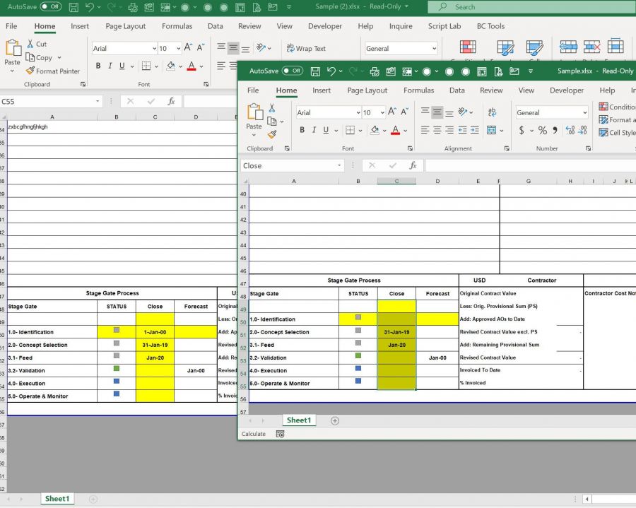
For example, the same cell is in 2 named ranges: C50 is in B50:D50 and C49:C55 named ranges. A change in cell C50 will highlight both ranges.

The code from the file attached will compare the names based on the first selected file and highlight the differences in both files.
Tip: you can go to your forum profile, and list the topics you have started (or posted into) to find one of your topics, you don't have to start a new one.
Hi Catalin,
Thank you for your reply and efforts.
What I intend to do is to highlight the data that exist in one sheet but not in the other, within each named range in both sheets.
The below code works perfectly for comparing two named ranges on my existing files on the same worksheet ...
Sub HighlightMissingData()
Dim rangeToUse As Range, singleArea As Range, cell1 As Range, cell2 As Range, i As Integer, j As Integer
Dim SelectionOne As Range, SelectionTwo As Range, WS1 As Worksheet, WS2 As Worksheet
Application.ScreenUpdating = False
ActiveWorkbook.Worksheets("Sheet1").Activate
Range("Ongoing_Activities, Outstanding_Activities").Select
Set rangeToUse = Selection
Cells.Interior.ColorIndex = xlNone
If rangeToUse.Areas.Count <= 1 Then
MsgBox "Please select more than one area."
Else
rangeToUse.Interior.Color = vbYellow
For i = 1 To rangeToUse.Areas.Count
For j = i + 1 To rangeToUse.Areas.Count
For Each cell1 In rangeToUse.Areas(i)
For Each cell2 In rangeToUse.Areas(j)
If cell1.Value = cell2.Value Then
cell1.Interior.ColorIndex = xlNone
cell2.Interior.ColorIndex = xlNone
End If
Next cell2
Next cell1
Next j
Next i
End If
End Sub
Hope that you can assist in showing the looping code that can perform this task.
Best Regards,
Zak
I don't understand your message.
I provided in previous message a file with the code that compares 2 files, the code will ask you to browse for the files.
Looks like you pasted your code again, even if you already did that twice before, without even testing the code provided.
Please test the file provided.
Hi Catalin,
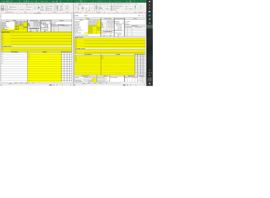
Before sending my previous message I tested the provided code and got the shown screenshot result. Please advise.

As mentioned, If the merged range has 10 cells, you cannot change the color to only one of them, you have to change the color to the entire merged range.
Try it yourself:
Merge some cells, then in vba run this code: ActiveCell.MergeArea.Cells(3).Interior.ColorIndex=6
It should highlight only the third cell, but you will not see any color in the merged range. If you unmerge the range, you will see color on third cell.
So it does not make sense to highlight only a cell in a merged range, you have to highlight the entire merged area if there is a difference between the 2 files for that range.
What the code does:
1. It will look into all sheets from the first file, then in all names from those sheets, and will check if the name exists in the second file.
2. If the name exists in both files, it will then check if the number of cells of that named range is equal in both files, if not it will highlight the named range, in both files
3. It will check all the cells from the named ranges, comparing them between files. If only one cell is different in that named range to the corresponding range from the second file, BOTH ranges are highlighted, not just that cell that is different, for the reasons described above.
if you want all cells to be highlighted separately, you have to move the lines that changes the color inside the loop, not outside the loop as it is now.
Many thanks Catalin for your very useful clarifications. As I am not experienced programmers I was just wondering, why the code I provided can do the proper highlight, as I just picked it from the web as it is?!
Thanks anyways for your efforts.
Then use the code you have.
I have not seen yet the RULES for "proper" highlighting.
You have to identify ALL possible scenarios and provide a RULE for each case, that is what you should do from the beginning.
These are the scenarios I see:
1. Named Range exists in both files, but:
1.a: the number of cells is not equal between the 2 files: WHAT needs to be done in this case? Does it make sense to compare them? What if 1 range has 3 cells and in the other file has 5 cells?
1.b: the number of cells is equal
1.b.1: all cells in the range are merged. This means that the merged range can only have 1 value, no matter how many cells are in the merged range. Highlighting cell 2 in a 10 cell merged range makes NO sense.
1.b.2: the cells from the named range are not merged. The code provided will still analize cell by cell, but if ONE cell is different than the one from the other file, all cells from the named range will be highlighted.
Identify all other possible scenarios and clarify WHAT needs to happen in each scenario.
