Hello all,

I am currently working on a digital rota for our company and have a bit of conditional formatting I want to apply to groups of cells. I have attached a sample spreadsheet for more clarity, but in a nutshell:

I have a group of cells E2:G3 (for one staff for Sunday for example) where
E2 (start time), F2 (end time) and G2 empty cell to mark with T for training, S for sick, AL for Annual leave, etc. E3 and F3 are for hours worked in a different department.

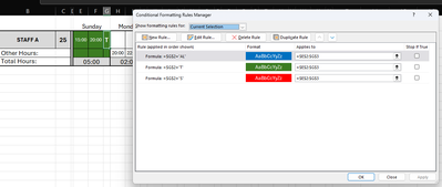
I have set up the conditional formatting as attached in the screenshot and everything works as predicted. When I enter one of the 3 codes in cell G2 the formatting is applied to all cells in E2:G3

Now I want the rest of the "groups" to work the same. So for all the other days and for the other staff that are identical in rows beneath. After googling and trying out various recommendations like the format painter and copy/paste special (formats) the results are not as wanted.
I also tried playing around with the absolution of the cell-references but again this throws up different results.

I do realise that I can copy/paste the blocks and then manually adjust the rules for each block in conditional formatting, but considering this rota consists of 3 weeks for 7 staff with each 3 rules to adjust it would be an enormous amount of work.

I might be clutching at straws, but I can't help to think that there might be a more elegant solution to solve this 😀 

Any help would be highly appreciated 😀 

Many thanks

Knut