Hello guys,
I have a really weird question to ask. Just coming here from " Interactive Excel Project Management Dashboard" video on Youtube, which was amazing.
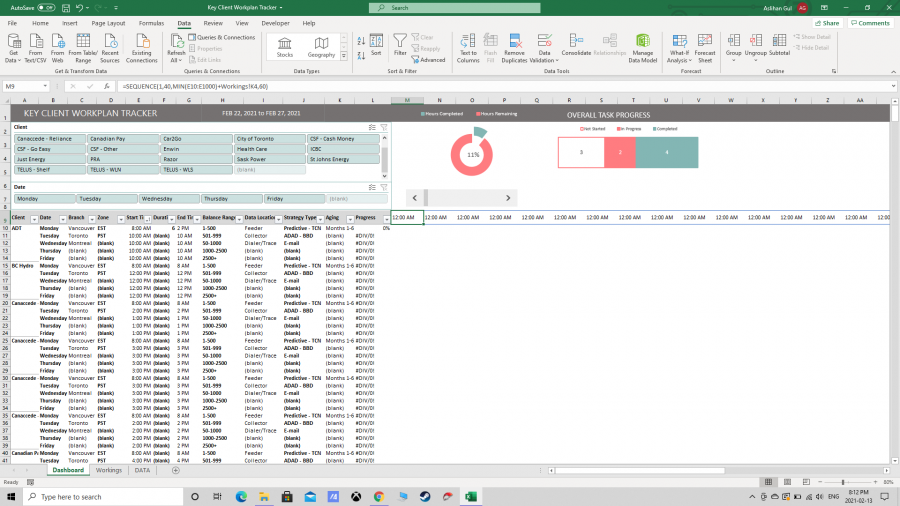
I've been trying to use Sequence formula for time just like Mynda used hers for date when she attached with scroll down and got her data from Pivot table. But mine is not seeing the time from my pivot table. I've tried everything but couldn't figure it out on my own. If you can help me, I would appreciate it. I'm trying to create a dynamic dashboard just like she explained on that youtube video.
Here is my dashboard and my formula. If you could help me figure it out, would be much appreciated!

Hi Aslihan,
Welcome to our forum! As I explained on YouTube, please provide a sample file so we can see what data you're working with in the PivotTable. The screenshot is illegible and even if we could read it, we would have to re-create your file to help you.
Thanks,
Mynda
I apologize for that. Here is my file and my data. I followed your way until the sequence formula but I must have did somethng wrong with the formula, it didn't work for Start time.
Thank you so much Mynda.
Asli
Thanks for sharing your file.
You can use this formula:
=SEQUENCE(1,40,MIN(E10:E1000)+Workings!K4*0.0416666666666667,0.0416666666666667)
Where 1 hour equals 0.0416666666666667
i.e. the time serial number for 1 hour.
Note: Your Start Time column contains blanks which equal zero, and your MIN cell range references through to row 1000 which also contains blanks which equal zero, so your time will always start at 12:00 AM which has a time serial number of zero.
Mynda
Oh my god!
Thank you so much. I am still in process of learning so never thought about 1 hour being 0.0416666666666667. I had those blanks for later to fill when we actually create the schedule but now I have filled them just to see, also fixed the cell reference until we have more data to add, now it works perfectly!
I really appreciate your help, you're such an amazing teacher and I can't explain how grateful I am for you.
I am also so glad that I found your video the other day so with that now I am part of this great community.
Thank you again,
Asli.
My pleasure, Aslihan 🙂
Hello Mynda me again,
I am still in the process of creating the dynamic dashboard. I have tried the Sequence formula which worked in my previous dashboard but I had to create another one and now I am having problem. It shows from 12 am even though I have deleted the blanks from my data and from my cell references. Trying this formula
=SEQUENCE(1,10,MIN(C10:C32)+Workings!E4*0.0416666666666667,0.0416666666666667).
Also I am trying to use the conditional formatting to see the schedule on the right sight, same as your video. I am trying the formula
=AND($B10=Workings!$G$5,L$9>=$C10,L$9<=$D$10) to compare the Task date to today's date(to see it on the day of the event) and the rest is based on the time but whatever I do, doesn't work at all.
Would you be able to help me with those? It would be much appreciated. Thank you so much
Asli
Hi Aslihan,
Right-click on the Start Date column in the PivotTable > Ungroup. This will fix the SEQUENCE formula. Repeat for the End Time column.
This should also fix the conditional format.
Mynda
