A few weeks ago one of our members, Kylie, sent me this question:
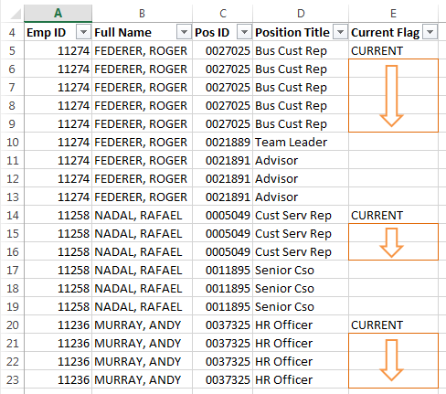
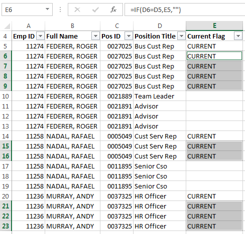
“How can I fill column E with the text ‘CURRENT’, if the Position Title in column D matches the first instance of ‘CURRENT’ in column E?”
See example data below; Kylie wants to fill the cells bordered in orange:
Note: I had to desensitise Kylie’s data and the first names that popped into my mind were inspired by the French Open. I hope Federer likes his new position as Business Customer Rep, or is that Bus Customer Rep…either way it’s going to be a big change for him 🙂
Download the Workbook
Enter your email address below to download the sample workbook.
Watch the Video
Fill Down based on Criteria
Unfortunately There's no IF option on the Fill tool but it's easy enough with a combination of Go To Special and an IF formula:
- Select the cells in column E from the first row of your data to the bottom of your data e.g. E4:E4000, but don’t select the whole of column E, you just want the rows containing data.
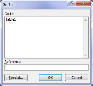
- Press CTRL+G to open the Go To dialog box > click the ‘Special’ button at the bottom:
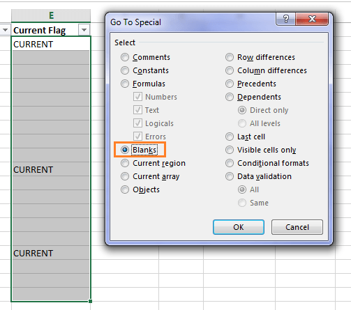
- Select ‘Blanks’ and click OK
This will have selected all blank cells in your data range in column E
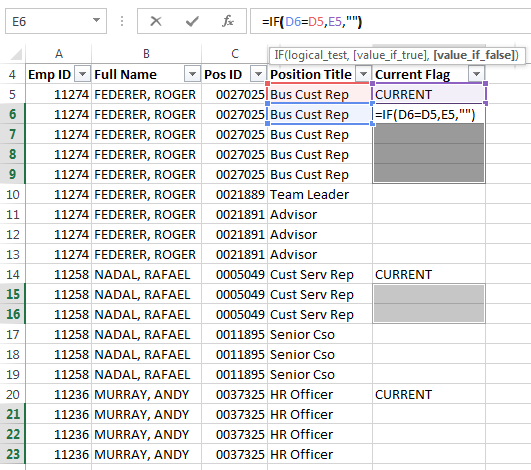
- In the formula bar enter this formula (assuming the first cell selected by Go To Special is cell E6, if not adjust cell references accordingly):
=IF(D6=D5,E5,"")
Let’s translate the formula into English:
IF the Position Title in D6 is the same as the Position Title in D5, then insert the Current Flag from E5, otherwise leave the cell blank.
- Press CTRL+ENTER to enter the formula in the selected empty cells
- Copy column E and Paste as Values to get rid of the formulas.
Note: if it was possible for Kylie's data to have the Position Title repeated for different employees you could make the formula an IF(AND... like so:
=IF(AND(D3=D2, A3=A2),E2,"")
This would also ensure the CURRENT flag was only copied down to the relevant employee.


Hello
I want Excel to recognise a delivery profile given as a number and to automatically use this number to populate cells beyond a given date with labour hours. For example, I have running horizontally 1 – 420 representing 420 months (35 years). There will be 120 products delivered commencing month 1 at a rate of 8 per month (15 month delivery program). The products will be subject to various maintenance interventions (e.g. every 4 years ‘A’ type exam, every 7 years ‘B’ type exam, every 10 years C’ type exam). Each exam requires a different amount of man hours to complete. On separate horizontal rows I would like Excel to recognise 1) When the exam type commences (and its multiples of), 2) to show in the respective horizontal row for the exam type the man hours for each month accounting for the delivery profile (e.g. ‘A’ type exam commences start of Year 4, and for 15 months thereafter man hours are shown for each month. Thank you
Hi Adrian, please post your question on our Excel forum where you can also upload a sample file and we can help you further.
I want to create small subset of my main humongous data base using two zip codes. I want all the columns of data in the main dataset in the smaller subset files. is there an equivalent of a “Select IF (VAR=”94110”) Then Write to (FILE) command and have it execute for every time the condition is true?
The Excel commands, I have looked at require me to define a range.
Hi Charles,
You could use Power Query to extract the data you want and save that into a table/tables in a file/files.
Without your data it’s difficult to give you a more complete answer. You cold start a topic on our forum and supply a sample file there, and we could give yo a better answer.
Regards
Phil
Can we achieve the same using query editor?
Yes. Please post your question and sample Excel file on our forum where we can help you further and our answers can also help others: https://www.myonlinetraininghub.com/excel-forum
Hello,
If values are changed in column “C” the formulas does not work.
How it is linked to formula? there is no reference in formulas from column “C”
would you please explain.
thanks
Hi Ahmed, change the formula to reference column C instead of D. If you’re still stuck please post your question on our Excel forum where you can also upload a sample file and we can help you further.
Saved me 5 hours, literally. Thanks!
Wow, that’s huge! Glad we could help 🙂
Hi Mynda, Would this formula be able to be re-worked to count the number of rows it fills with “CURRENT” (e.g. 139) and fill to a certain number (e.g.160)?
Hi Angelique,
Can you post sample data file on our forum? It will be easier to see what you’re after. (create a new topic after sign-up)
Catalin
just great
🙂 Thanks, Maggie!
Nice to check it on youTube. Thanks for sharing the knowledge.
You’re welcome, Purushottam 🙂