Smart Excel Checklist

Most to-do lists fail for one simple reason: they rely on manual effort to stay accurate.

In this tutorial, you’ll build a smart Excel checklist that:

• Automatically prioritises tasks based on due dates
• Visually separates urgent, upcoming, and completed tasks
• Tracks overall progress with a dynamic progress bar
• Updates instantly as you tick items off
• Requires no VBA or macros

You can use this system for product launches, content calendars, event planning, personal goals, or team projects, anything with tasks and deadlines.

Watch the Step-by-step Video

Download the Practice File

Step 1: Create the Checklist Table

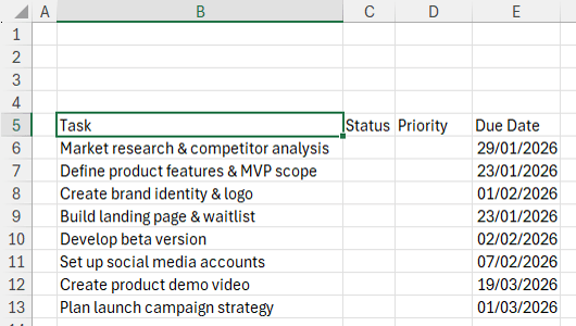
1. Set up the headers

Enter the following headers:

• Task
• Status
• Priority
• Due Date

This structure works for any type of checklist, including:

• Content calendars
• Event planning
• Wedding tasks
• Personal goals
• Team projects

Feel free to rename or add columns if needed.

2. Enter tasks and due dates

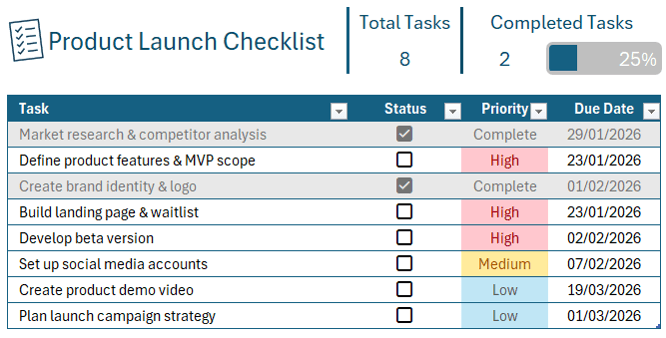
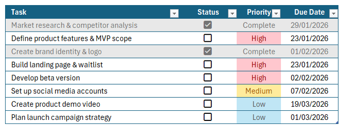
Add a list of tasks in the Task column, such as:

• Market research and competitor analysis
• Define product features and MVP scope
• Create brand identity and logo
• Build landing page and waitlist
• Develop beta version
• Set up social media accounts
• Create product demo video
• Plan launch campaign strategy

Then enter corresponding Due Dates for each task. Your table should look like this so far:

3. Convert the range into an Excel Table

Excel Tables make this entire system work smoothly.

1. Click any cell in your data range
2. Press Ctrl + T
3. Confirm My table has headers, then click OK

Next, rename the table:

• Go to the Table Design tab
• Change the table name to Tasks

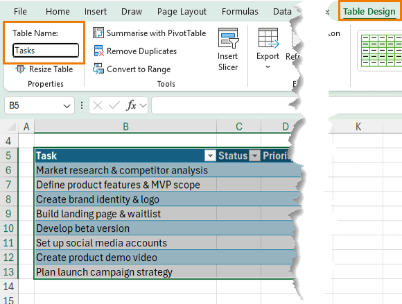
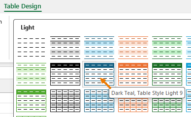
From the Table Style gallery apply any table style you like. A darker style works well because it improves contrast for conditional formatting later.

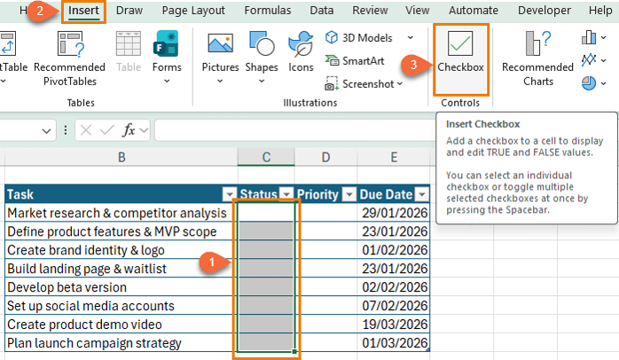
4. Add checkboxes to the Status column

1. Select the Status column
2. Go to the Insert tab
3. Choose Checkboxes

Each checkbox stores an underlying value:

• Checked = TRUE
• Unchecked = FALSE

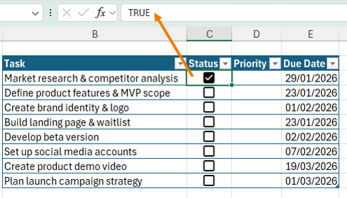
These values will drive your formulas and progress tracking.

Step 2: Auto-Assign Priority Based on Due Date

Instead of manually tagging tasks as high or low priority, you’ll let Excel decide based on deadlines.

Priority logic

Use the following rules:

• Completed if the task is checked off
• High if due in 7 days or less
• Medium if due in 14 days or less
• Low if due later than 14 days

Enter the priority formula

In the Priority column, enter this formula:

=IFS(
    [@Status],"Complete",
    [@[Due Date]]-TODAY()<=7,"High",
    [@[Due Date]]-TODAY()<=14,"Medium",
    TRUE,"Low"
    )

What this does:

• Checks the Status column first
• Uses today’s date to calculate urgency
• Returns priority labels automatically
• Copies down instantly because it’s inside a Table

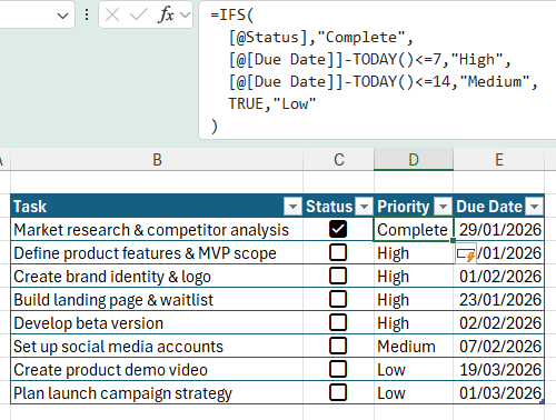
The table’s structured references used in the formula e.g. [@Status] make the formula easier to read and maintain.

Step 3: Add Visual Completion and Priority Effects

Now you’ll use Conditional Formatting to make the checklist visually intuitive.

Highlight priority levels

1. Select the Priority column
2. Go to Home > Conditional Formatting > Highlight Cells Rules > Text that Contains

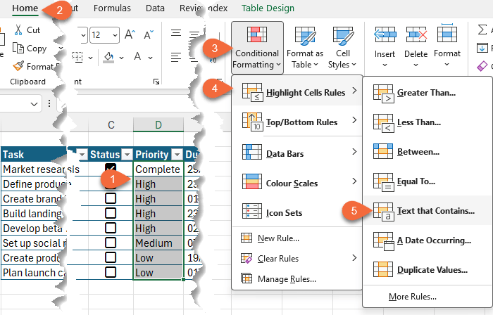
Apply these formats:

• High
  • Light red fill with dark red text
• Medium
  • Yellow fill with dark yellow text
• Low
  • Custom format with blue font and light blue fill

Fade completed tasks

To de-emphasise completed work:

1. Select the entire table excluding the headers
2. Go to Home > Conditional Formatting > New Rule
3. Choose Use a formula to determine which cells to format
4. Enter this formula (adjust the column if needed):

=$C6

This checks whether the checkbox is TRUE.

Apply formatting:

• Grey fill
• Grey font

Completed tasks now fade into the background while active tasks stand out.

Step 4: Track Progress Automatically

At this point, the checklist already:

• Updates priorities automatically
• Highlights urgent work
• Fades completed tasks

Now let’s add a progress tracker.

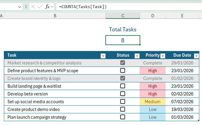
Count total tasks

• In Cell C2, enter: Total Tasks
• In Cell C3, enter:

=COUNTA(Tasks[Task])

This counts all tasks and automatically updates if new ones are added:

Count completed tasks

• In Cell D2, enter: Completed Tasks
• In Cell D3, enter:

=SUM(--Tasks[Status])

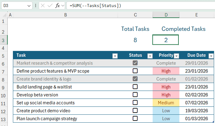
Why this works:

• TRUE equals 1, FALSE equals 0
• The double unary (--) converts TRUE/FALSE into numbers
• SUM adds up completed tasks instantly

Calculate percentage complete

In Cell E3, enter:

=D3/C3

Format the cell as a percentage.

Add a progress bar

1. Select Cell E3
2. Go to Conditional Formatting > Data Bars
3. Open Manage Rules and edit the rule

Set:

• Minimum = 0
• Maximum = 1
• Bar colour to match your theme

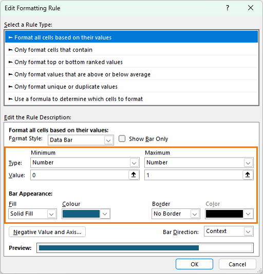
Optional finishing touches:

• Grey cell fill
• White font
• Add a rounded rectangle shape over the bar (hold Alt to snap to grid)

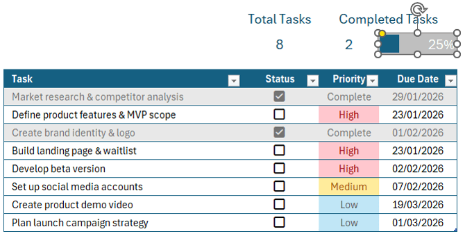
Step 5: Final Polish

• Add a title such as Product Launch Checklist
• Insert a checklist icon and match its colour to your theme
• Add borders around the summary metrics
• Align and space elements for clarity

Test the System

Try the following:

• Tick off a few tasks
• Change a due date to an earlier date
• Add a brand-new task

You’ll see:

• Priorities update automatically
• Completed tasks fade
• The progress bar adjusts instantly

This approach is more reliable than manual tagging because:

• Dates don’t lie
• Urgency updates automatically
• Your checklist stays accurate with zero extra effort

Want to Go Further?

What you just built uses Excel Tables, formulas, and conditional formatting; some of Excel’s most powerful features.

If you want to master these skills properly, check out the Excel Expert course, where you’ll learn:

• Advanced formulas and functions
• Conditional formatting mastery
• Excel Tables
• PivotTables
• And much more

All taught with real-world examples, not theory.