Searchable Drop Down List in Excel

Creating this searchable drop down list in Excel is so easy I’m wondering why I never thought of it before. It doesn’t require any formulas or VBA and it has all the bells and whistles you’d expect from a searchable drop down list, including automatic sorting, ignoring duplicates and an option to select ‘All’:

Watch the Video

Download Workbook

Searchable Drop Down List in Excel Instructions

This technique couldn’t be simpler.

Step 1: Insert a PivotTable

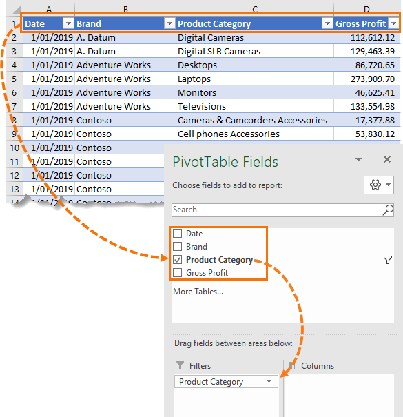
Your searchable drop down list can be based on a single field (column) in a larger table, as in my example, or it could simply reference a single column of data. Note: Make sure your data has a header row.

Select your table, or a cell in the table > Insert tab > PivotTable. Choose where you want the PivotTable placed (this will be the cell that contains your searchable drop down list).

Step 2: Add Field to Filter Area

The fields available in the PivotTable field list are the column labels from your data. Drag the column/field you want your searchable drop down list based on into the Filter area of the PivotTable.

Step 3: Format PivotTable Style (Optional)

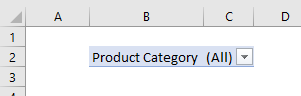
By default, PivotTables have a blue colour format:

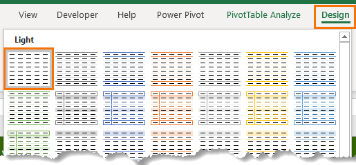
However, you may prefer to set the style to something more subtle via the PivotTable Design tab:

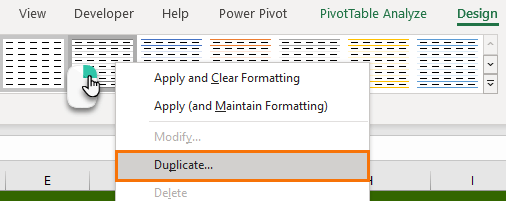
Tip: You can create your own custom style with no formatting by right-clicking the second style > Duplicate:

In the Modify PivotTable Style dialog box that opens, you can clear the formatting as required:

Step 4: Link a Formula

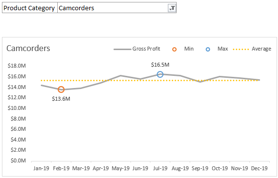
One use for this searchable drop down list is to reference it in a formula. In my example I used it with SUMIFS to build a table that I linked to a regular chart, which you can see below. Notice that it includes highlighting of the minimum and maximum and displays the average. All features not possible with a Pivot Chart.

Limitations

Although I love this method for creating a searchable drop down list in Excel, it still comes with some limitations.

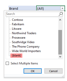
1. It won’t ignore blanks in your dataset. It’ll show them as (blank) at the end of the list:

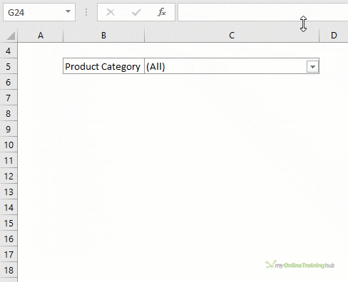
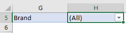
2. It’s not suited to using as a data validation list for data entry in a table because it requires two cells, one for the field name and one for the item (shown below in cells G5 and H5 respectively):

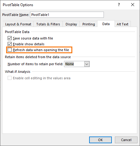
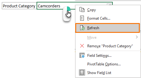
3. It requires a Refresh of the PivotTable for any new items to appear in the list. I personally don’t think this is a big deal because you can set the PivotTable to automatically refresh upon opening the file in the PivotTable Options available in the right-click menu:

Or right click the PivotTable > Refresh: