In Australia we did away with 1 and 2 cent coins years ago. So all prices, where paid in cash, are rounded down to the nearest value divisible by 5 cents.
In Excel we can use the FLOOR function to calculate this value. For example:
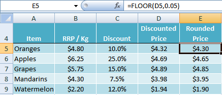
Say our price is $4.32 and we need to round it down to the nearest value divisible by 5 cents, the FLOOR function would read:
=FLOOR(4.32, 0.05)
= $4.30
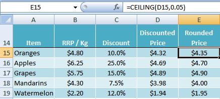
On the flip side we could use the CEILING function to round our price up to the nearest 5 cents as follows:
=CEILING(4.32, 0.05)
= $4.35
How do the FLOOR and CEILING Functions Work?
The syntax is:
=FLOOR(number, significance)
=CEILING(number, significance)
Where the number is your starting point and the significance is the multiple you want your number rounded down to for FLOOR, or up to for CEILING.
Unlike ROUNDUP or ROUNDDOWN, Excel’s FLOOR and CEILING functions can round the decimal places of a value to be divisible by a number you specify.
FLOOR Function Cool Trick
You’ve probably noticed that ‘7’ is the new ‘9’; with prices like $9.97 now in place of $9.99, and $9.47 in place of $9.49. So what if you wanted to round your prices to end in 47 cents or 97 cents?
We can use a combination of the FLOOR function and an IF statement to achieve this.
In row 25 in the example below you can see in the formula bar we have used the following formula:
=FLOOR(D25,1)+IF(CEILING(D25,1)-(D25)<0.5,0.97,0.47)
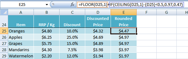
Taking row 25 as an example let me break this formula down and explain it in English:
1. The first part
=FLOOR(D25,1)
simply gets rid of the decimal places so you’re left with $4.00.
2. The second part
IF(CEILING(D25,1)-(D25)<0.5,0.97,0.47)
works out if the cents are less than 50, and if they are round them down to 47 cents, otherwise round them up to 97 cents.
3. The plus sign in between the first FLOOR function and the IF Statement adds the two results together giving the result $4.47.
Enter your email address below to download the sample workbook.


Hello Mynda
Thank you very much for this VERY useful tutorial and thank you to all the responders with their unique scenarios and solutions.
I was encountering the problem with your original formula of items priced $2.09 would round up to 2.49 instead of 1.99 which we prefer in our store to be more competitive. I ended up using @Siôn formula to help facilitate and it is successfully in those instances where items are priced closer to 1.99.
Although for items at 7.34, I need to use @Mynda formula to get to 7.49.
Do you know how I could combine your 2 formulas?
Thank you Mynda and Siôn
Hi Daniel,
It sounds like you have some special rules like the 7.34 rounding to 7.49 etc. Please post your question on our Excel forum where you can also upload a sample file showing all scenarios and your desired result and we can help you further.
Mynda
hi, please help me, IN excel i want both if 17.4 it should be round to 17, and if it is 17.6 it should become 18, i want single formula
Try:
=Round(A1,0)
in an excel round off at a rate of 50 paise is less than fifty paise below zero (eg.Rs.2147.41 is round off Rs.2147 & Rs.2147.52 is round off Rs.2148)
which formula apply this for an excel
pls help me
thanks
Hi Jayasree,
Use a simple Round function, to 0 decimal places:
=Round(A1,0)
In your cool trick, couldn’t you just use the following?
=CEILING(D25,0.5)-0.03
Not quite, Charles. If the value in D25 is 4.32 your formula still returns 4.32.
I agree with Charles. CEILING(4.32,0.5) = 4.50, and 4.50-0.03 = 4.47. So I don’t see how his formula isn’t perfect. Were you perhaps thinking of CEILING(4.32,0.05) instead — i.e. rounding up to the nickel instead of the half dollar?
Hi David,
I assumed Charles was referring to the rounding to .47 or .97 scenario, but his formula didn’t solve either. =CEILING(4.32,0.5) = 4.35, not 4.50.
Mynda
Is it possible there is some regional setting on your computer that is creating the difference because that formula absolutely resolves to 4.50 using both CEILING and CEILING.MATH.
$4.32 $4.50 =CEILING.MATH(A1,0.5)
$4.49 $4.50 =CEILING.MATH(A2,0.5)
$4.50 $4.50 =CEILING.MATH(A3,0.5)
$4.51 $5.00 =CEILING.MATH(A4,0.5)
Versus…
$4.32 $4.35 =CEILING.MATH(A6,0.05)
$4.49 $4.50 =CEILING.MATH(A7,0.05)
$4.50 $4.50 =CEILING.MATH(A8,0.05)
$4.51 $4.55 =CEILING.MATH(A9,0.05)
Therefore…
$4.32 $4.47 =CEILING.MATH(A11,0.5)-0.03
Hi David,
Not that I’m aware of. The example on Microsoft’s website also says 4.42 will round to the nearest nickel.
Do you want to share your file on our Excel Forum and include a screenshot in the file of how it appears to you so I can test it on my PC?
Mynda
I don’t think posting a file or screen shots will be necessary because the example from Microsoft is using this formula: =CEILING(4.42,0.05). Note that’s zero point zero five — i.e. five cents or one nickel. Whereas Charles and I have been proposing =CEILING(4.42,0.5), which is zero point five or zero point five zero if you prefer — i.e. fifty cents or half a dollar. And that’s the critical difference — 0.05 versus 0.50. So our formula rounds to the nearest half dollar and then subtracts three cents so that everything rounds to 47 or 97.
Right you are, David. It appears I could not see the ‘0’ for the trees! 🙂
Hi there, and thank you for this great material.
Regarding the cool trick, maybe not so cool but shorter using ROUND:
=IF(D25<0.5,0.47,ROUND(D25,0)-0.03).
What do you think?
Hi Siôn,
Thanks for sharing your formula. I get $3.97 for row 25 so I think you need to build in some more logic to handle values that end in the range .01 to .49.
Mynda
That is great tips. I may change your formula to remove ‘CEILING’ part. See below,
=FLOOR(D25,1)+IF((D25-FLOOR(D25,1))<0.5, 0.47, 0.97). What do you think?
Thanks,
Jon
Thanks, Jon. Swings and roundabouts I think 🙂
Cheers,
Mynda
I am looking for a way to round up to the nearest .05. If the price already ends in a 0 or 5, I would like it to remain and not round up. I can’t seem to figure out how to do this consistently. It seems the price will stay in some instances and in others, it rounds up. Any tips? Thanks!
Hi Victoria,
This is the quickest I could get back to you:
=IF(OR(A1-INT(A1) = 0,A1-INT(A1) >0.05),A1,CEILING(A1,0.05))
There may be other workarounds.
Here’s the Pseudo-Formula
=IF Decimal is is 0 or Greater than .05 then
Decimal stays the same.
for i.e. 4.00 = 4.00
4.06 = 4.06
4.056 = 4.056
IF Decimal is .01 to .05 then
it’s rounded up to .05
for i.e. 4.02 = 4.05
Now this may not be what you desire So I would gladly appreciate any further clarification.
Read More on Ceiling and Floor Functions
Rounding Off Numbers
Thanks.
CarloE
Thank you, I appreciate the response.
This did help. However, not in all cases.
If the decimal is greater than .05 then I want it to round up. I have listed examples of how I would like the rounding to go below. Basically, I have a set of prices that are derived from a separate formula. I want these prices to all stay where they are if they end in a 5 or zero. But, if they do not I would like them to round up.
3.60 = 3.60
3.65 = 3.65
3.67 = 3.70
3.61 = 3.65
I have tried to edit the formula you so kindly sent, but I am not having any success. I would appreciate any further guidance you could provide. Thanks!
Hi Victoria,
Sorry for that. Anyway now that it is clear… here it is:
=IF(INT(RIGHT(MOD(A1,1),1))<=5,ROUNDDOWN(A1,1)+0.05,ROUNDUP(A1,1)) or =IF(INT(RIGHT(A1-INT(A1),1))<=5,ROUNDDOWN(A1,1)+0.05,ROUNDUP(A1,1)) The Formula is simple: If the decimal tenths is a 5 or less then stays 5 else rounded up to the nearest decimal ones or rounded up to zero i.e. .05 is to .10 Note: Mod extracts the decimals out of a given number Right isolates the tenths place which is 5 Rounddown rounds down to the next lowest decimal ones + .05 RoundUp rounds the number up to the nearest decimal ones Sincerely, CarloE
Your “neat trick” could cause major damage to legal health! See S18 Consumer and Competition Act 2010.
Your column B quotes a discount.
With Oranges, Apples, and Grapes the rounded price is now LESS than the discounted price.
If you publicise your discount, your rounded price in those three cases will be misleading or deceptive conduct unless you use “Up to 10% off” system.
😀 Funny!
Thanks, Norman.