Want to turn your messy customer spreadsheets into a powerful, searchable CRM, right inside Excel? In this step-by-step tutorial, you'll learn how to use Power Query custom data types to combine customer details, interactions, and opportunities into a sleek, self-updating Excel CRM dashboard.
No VBA. No add-ins. Just Excel for Microsoft 365.
Table of Contents
- Watch the Excel CRM Step-by-step Video
- Get the Excel CRM Template and Practice Files
- What You'll Learn
- Why Build a CRM in Excel?
- Step 1: Prepare Your CRM Data
- Step 2: Import the CRM Tables via Power Query
- Step 3: Create Custom Data Types in Power Query
- Step 4: Build the Customer Details Report
- Step 5: Display Customer Interactions
- Step 6: Build the Active Leads Report
- Step 7: Filter and Refresh
- Real-World Use Cases
- Want to Learn More?
Watch the Excel CRM Step-by-step Video

Get the Excel CRM Template and Practice Files
Enter your email address below to download the free file.

What You'll Learn
- How to import multiple CRM tables into Power Query
- How to create custom data types for customers, interactions, and opportunities
- How to use formulas to extract customer details and filter active leads
- How to build a CRM that updates automatically as your data grows
Why Build a CRM in Excel?
Excel remains one of the most flexible and accessible tools for managing business data and with Power Query custom data types, you can compress entire records into single cells and then pull out just the fields you need, with ease.
That means less clutter, more control, and better performance.
Step 1: Prepare Your CRM Data
My example has three tables (all in Excel format) but you can have more or less:
- Customers: Name, Industry, Email, Country, Status
- Interactions: Date, Channel, Topic, Outcome
- Opportunities: Stage, Value, Expected Close Date
You can store these tables in one file, multiple files, or even connect to a database. Power Query handles them all.
Step 2: Import the CRM Tables via Power Query
1. Go to Data > Get Data > From File > From Workbook (or chose the appropriate source for your data)
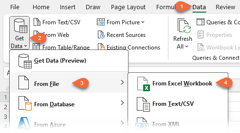
2. Browse to your file and check "Select multiple items"
3. Select the tables: Customers, Interactions, and Opportunities
4. Click Transform Data
This opens Power Query Editor.
Step 3: Create Custom Data Types in Power Query
For each table:
1. Select all columns
2. Right-click > Create Data Type
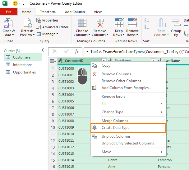
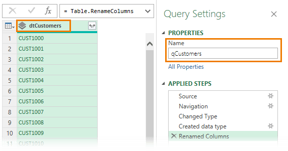
3. Rename the resulting column for each table:
- dtCustomers
- dtInteractions
- dtOpportunities
4. Rename each query for clarity:
- qCustomers
- qInteractions
- qOpportunities
Then go to Home > Close & Load To > Only Create Connection
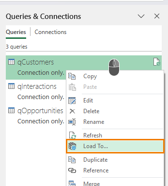
Right-click each query in the Queries & Connections pane > Load To > Table (on the same worksheet if desired)
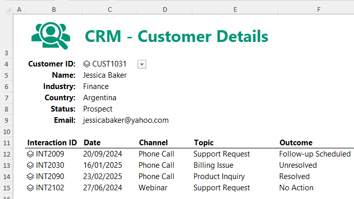
Step 4: Build the Customer Details Report
Create a new worksheet with this layout:
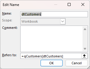
Create the Drop-Down List
1. Define a name (Formulas tab > Define name):
2. dtCustomers = qCustomers[dtCustomers]
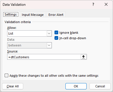
3. In cell C4, use Data Validation > List
Source: =dtCustomers
Extract Customer Details
Use dot notation to pull fields from the custom data type in cell C4:
Name: =IFERROR(C4.FirstName & " " & C4.LastName, "Select Customer ID")
Industry: =IFERROR(C4.Industry, "Select Customer ID")
Country: =IFERROR(C4.Country, "Select Customer ID")
Status: =IFERROR(C4.Status, "Select Customer ID")
Email: =IFERROR(C4.Email, "Select Customer ID")
Now, changing the customer ID in the dropdown instantly updates the report.
Step 5: Display Customer Interactions
Add this section below the customer details:
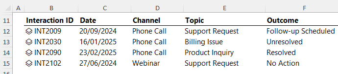
Use this formula to filter interactions for the selected customer:
=FILTER(qInteractions[dtInteractions], qInteractions[dtInteractions].CustomerID = C4.CustomerID, "No records")
Extract fields from the spilled array:
Date: =IFERROR(B12#.Date, "")
Channel: =IFERROR(B12#.Channel, "")
Topic: =IFERROR(B12#.Topic, "")
Outcome: =IFERROR(B12#.Outcome, "")
Step 6: Build the Active Leads Report
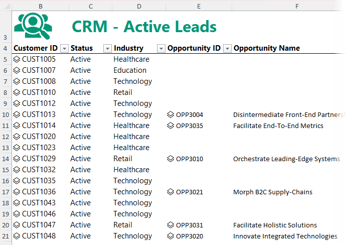
Create a new sheet with these columns:
- Customer ID
- Status
- Industry
- Opportunity ID
- Opportunity Name
- Stage
- Value
Get Active Customers
=FILTER(qCustomers[dtCustomers], qCustomers[dtCustomers].CustomerStatus="Active", "No active leads")
Extract Details
Status: =IFERROR(B5#.CustomerStatus, "")
Industry: =IFERROR(B5#.Industry, "")
Match Opportunities
Opportunity ID: =XLOOKUP(B5#.CustomerID, qOpportunities[dtOpportunities].CustomerID, qOpportunities[dtOpportunities], "")
Then use dot notation to display opportunity fields:
Opportunity Name: =IFERROR(E5#.OpportunityName, "")
Stage: =IFERROR(E5#.Stage, "")
Value: =IFERROR(E5#.Value, "")
Step 7: Filter and Refresh
Apply Excel filters to slice by:
- Industry (e.g. Technology, Finance)
- Stage (e.g. Qualified, Proposal, Negotiation)
To update everything, just go to Data tab > Refresh All.
Your CRM now grows with your data — no manual editing required.
Real-World Use Cases
Besides a CRM, Power Query custom data types can be used for:
- Product catalogues
- Bills of materials
- Employee databases
- Support ticket dashboards
- Inventory systems and more
Want to Learn More?
If you found this helpful and want to master Power Query and Excel automation, check out my full Power Query course. Thousands of professionals have already used these techniques to build tools they actually use.
See all Excel course options here.

Absolutely love this. I’ve also looked into your video on “Automated Database entry’. I would love to see these two combined.
As a question though, what process is there to update a field like email etc. to account for changes or entry errors? Is there something beyond going all the way back to the Data table?
You could build a form that you can use to search for and recall an entry, then allow you to edit it and write it back to the database.
Great video, thanks for sharing.
Have you noticed that YouTube has taken this video down because it violates YouTube’s policy on harassment and bullying which makes no sense.
Thanks, Sam. Yes, we’re aware of the video being removed from YouTube. This was because the dummy example data looked too realistic so they though I was sharing real email addressed.
It would be interesting to see how this solution handled multiple Opportunities per Customer. We normally have many running at the same time. Does your course handle something like that?
Hi Trishia,
Yes, you can use the same technique I used to show multiple interactions, to show multiple opportunities.
Mynda
I would love to see how that is done because as I am looking at it I can’t get it to show any past the first Opportunity or Interaction. 🙁
I show you in the first example where I retrieve the interactions. Copy the CRM Customer Interactions sheet and edit the formula to change the table being looked up from Interactions to the Opportunities. If you’re still stuck, please post your question on our Excel forum where you can also upload a sample file and we can help you further.
Always great information and presented in a very understandable format. I’ve been using Excel ( Lotus123) for 35 years. Wish this was was available then!, thank you!
Cheers, Jack! Glad you enjoyed it.