
You’re not likely to hear about Excel’s Camera tool on a training course and you certainly won’t find it on the ribbon. It is one of those insider tips that are hidden away in the toolbar options.
What is Excel’s Camera Tool
The camera tool takes a snapshot of a range of cells from somewhere else in your workbook and displays it where ever you position it. The snapshot image dynamically updates so when the data changes, the snapshot changes too.
Add Excel’s Camera Tool to Your Quick Access Toolbar
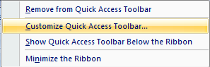
1. Add the camera tool to your Quick Access Toolbar. Right click on the Quick Access Toolbar and select ‘Customize Quick Access Toolbar’.
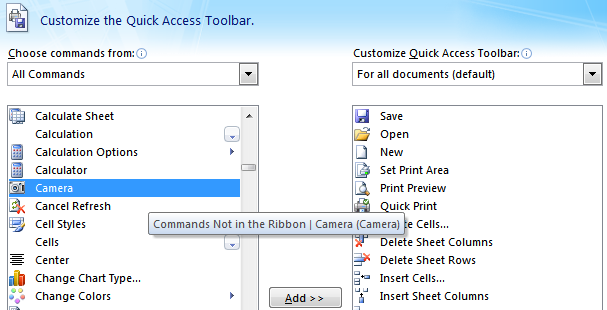
2. You’ll find it under ‘All Commands’, then scroll to ‘C’ for Camera. Click ‘Add’ to add it to your Quick Access Toolbar.
How to Use Excel’s Camera Tool
1. Select the cells you want displayed in your snapshot. Note: if you’re taking a snap shot of a graph you will need to align the graph to the underlying cells first.
2. Click the Camera icon on your Quick Access Toolbar.
3. Click the worksheet location you want your snapshot placed.
4. Use the handles to resize and reposition it.
5. Right clicking the image brings up options for formatting the snapshot like removing borders, cropping, protection etc.
Handy Uses for Excel’s Camera Tool
1. It’s handy for putting together dashboards as you can resize the snapshot to fit where you choose.
2. If you don’t have the luxury of two monitors you can take a snapshot of the result area of your workbook that you want to monitor or reference and insert it on the sheet you are working on.
Advanced Camera Tool Tip – Use IF Statements to Determine What Cell Range to Display
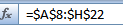
When you click on your snapshot image you’ll notice in the formula bar that it is referencing the range of cells displayed in the snapshot.
This means you can use an IF statement to determine what range of cells the snapshot image displays.
For example; if results are favourable use the graph with green colour formatting, but if the results are negative use the graph with red colour coding.
Unfortunately you can’t write a standard IF statement that references cell ranges e.g. $C$1:$G$50, you have to use Named Ranges, but this is a minor inconvenience.
For detailed instructions on how to use formulas with your camera tool check out Charley Kid’s tutorial.
Limitations of Excel’s Camera Tool
1. The image doesn’t stay sharp when you reduce it significantly.
2. The camera images don’t print well, so it’s really only ideal for viewing on screen.
Want More Tips Like This?
Tips That Make Your Work Easier, Faster
And Much More Enjoyable!
Click Here to Get 102 Excel Tips & Tricks


 Microsoft Excel’s N Function

Margaret Pont
Fantastic information, as always. Kind regards
Maggie
Philip Treacy
Thx Maggie
VV
Hi Mynda,
When I read the camera feature article, I was ecstatic! It was exactly what I was looking for but I am having a some trouble. I tried using the IF function with name ranges however it is not working. The formula I am using is =IF($B$43=”ON”,OntarioWaterfalls,QuebecWaterfalls) but it is giving me an error message saying, “This formula is missing a range reference or a defined name”. Do you know what I could be doing wrong?
Thank you for all your wonderful tips always!
Mynda Treacy
Hi VV,
It’s difficult to say without seeing your file, but the error suggests that you haven’t set up the named ranges. If that’s not it, please post your question and Excel file on our forum where we can help you further.
Mynda
Mitch
Hi,
I’ve always been using the camera tool for various reports, but there is one thing i can’t figure out and maybe you can help me with it. When you create image with the camera tool, sometimes the image will resize when you adjust column heights/row heights or insert rows/columns within the target range. Sometimes, it will not resize the image and simply shrink the image inside. I have played with various property of the image but cannot figure out how to toggle between the two (and even if the image was initially resizing, after a while it reverts back to not resizing). Any idea?
Mynda Treacy
Hi Mitch,
I don’t use the camera tool all that much. can you please share a sample file on our Excel Forum so we can replicate the issue and try to understand more about it?
Mynda
Joan Hauff
I have been using Excel daily for years and never knew about the Camera tool. Thanks.
Mynda Treacy
Yes, there seems to always be something new to discover in Excel 🙂
wilson
like the camera tool only seem it one other place USEFUL
GULZAR
if any book of vba userform training kindly send me.your book of 100 excel tips and tricks is very useful and your way of teaching is so nice.thank
Mynda Treacy
Hi Gulzar,
Glad you liked the 100 Excel Tips and Tricks eBook. Unfortunately we don’t have one for VBA.
Kind regards,
Mynda
Wanda Ponto
What is the difference between the Camera Tool versus the Paste > As Picture > Paste Picture Link? This dynamically updates as well.
Thanks
Mynda Treacy
Not much, the Paste Picture Link is a new feature in Excel 2007 (I think).
putra
Hello Mynda,
Thanks for the sharing.
Btw kindly please advise whether this camera tool can be use to display the hidden cell ? Thanks in advance.
best regards,
putra
Mynda Treacy
Hi Putra,
No, the camera tool displays the cells based on their size. If you hide the cell(s) (row/column) the cell effectively has 0 size and the camera doesn’t display anything.
Cheers,
Mynda.
yaser
Dear mynda,
u r great!!!
can u help me ,i cannot make camera image for a graph?
pls.advise
regards,
yaser
Mynda Treacy
Hi Yaser,
If you follow the numbered steps in the tutorial above it explains what do to to take a camera snap shot of your graph. If you get stuck you can send your workbook to me via the help desk.
Kind regards,
Mynda.
Stephen Moore
Re: Printing Limitations
You can make camera objects print properly with a couple of refinements.
Firstly, you need to make an input cell, with a value of TRUE or FALSE. This could just be a drop-down list for ease of use.
Then, set a named range for the cells you want a picture of, which Refers to =IF([input cell],[cells you want],””). When you have FALSE selected the camera will not update for the named range, and the picture will print normally.
Mynda Treacy
Nice trick. Thanks, Stephen 🙂
reza
hi dear
Iam reza
i read this page and learn from U
great thanks
Mynda Treacy
Thanks, Reza 🙂
Raymond Gota Toudji
Dear Mynda,
Just read your e-book.
It has great stuff, is well presented and nicely explained!
Thanks for sharing, and I’ll definitely pass it through.
I also like the layout of your site.
Regards,
Raymond.
Mynda Treacy
Thanks. Raymond 🙂 I appreciate you taking the time to share your feedback.
Joseph Horling
Hi Mynda,
I was just messing around with the Camera in Excel. I took a snapshot of one of my data tables and placed it in another Sheet. When I updated the original date adding another row of data the snapshot did not dynamically update. Can you show me how to do this? Thanks, Joe.
Mynda Treacy
Hi Joseph,
It should automatically update. I tested it in Excel 2007 and 2010 and it updates by default for me. What version of Excel are you using?
Kind regards,
Mynda.
Joseph Horling
Hi Mynda, I am using Excel 2010 version. Added another row of date to the table. It updated the dashboard, but not the snapshot. I must be doing something wrong, not sure. Joe.
Mynda Treacy
Hmmm. I’m not sure either. Can you send me the file via the Help Desk and I’ll try on my PC?
Joseph Horling
Hi Mynda, Submitted a ticket request at the help desk. joe
Mynda Treacy
Hi Joseph,
Ok I got your file, thanks. I presume you mean when you add rows to your table on sheet1 the picture doesn’t update? Because when I change a value in any of the cells of the existing table the picture does update.
So, when you insert a picture it actually links to a specific range of cells. If you select the picture object and look in the formula bar you can see the range of cells the picture is referring to.
Your picture only picks up the table cells originally referenced when inserting it, it doesn’t detect that more cells have been added to the table and grow accordingly.
There doesn’t appear to be a solution to this (I’ve read elsewhere that this is a limitation in Excel 2007 onwards), however if you change the range your picture is linked to to make it bigger than the table, and insert rows within this range the picture does grow, just like a range referenced in a formula would grow when inserting rows within it.
e.g. range is Sheeet1!$A$1:$E$25 if I insert a row above row 25 my range grows to Sheeet1!$A$1:$E$26
So, instead of typing in new data in the first blank row under your table, you will need to insert a row first, then type your data so that your picture link increases. Not ideal, but all I can think will work.
I hope that helps.
Kind regards,
Mynda.