Excel CHOOSE Function

Excel’s CHOOSE function is not much use on its own, but when you nest it with other functions it can make quite a difference to their capabilities.

First let’s look at the basics of the CHOOSE function.

CHOOSE syntax:

=CHOOSE(index_num, value1, value2, value3…..up to 254 values)

With an example:

=CHOOSE(3,“ Blue”,”Green”,“Orange”)

Translated the formula reads:

=CHOOSE(value number 3 where, value 1 = Blue, value 2 = Green, value 3 = Orange)

The result is Orange

CHOOSE Function Examples:

1.       The index number can be a number or a reference to a cell that contains a number up to 254. E.g.

=CHOOSE(A1,“ Blue”,”Green”,“Orange”) where A1 contains the number 2 will return ‘Green’.

2.       If the index number is less than 1 you will get a #VALUE! error. E.g.

=CHOOSE(0.5,“ Blue”,”Green”,“Orange”) you will get a #VALUE! error.

3.       If the index number is more than the number of values you have you will get a #VALUE! error. E.g.

=CHOOSE(4,“ Blue”,”Green”,“Orange”) you will get #VALUE!

4.       If the index number is not an integer or whole number it will round the number down to the nearest whole number. E.g. 2.95 will be translated to 2. E.g.

=CHOOSE(1.5,“ Blue”,”Green”,“Orange”) you will get ‘Blue’.

5.       The values can also be cell references e.g.

=CHOOSE(3, A3,A4,A5) you will get ‘Orange’.

Advanced uses for the CHOOSE function

1.       Use it with SUM. In row 13 below you can see the formula that is used in row 12.

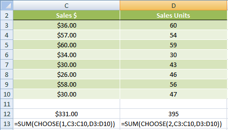Effectively these formulas are performing a simple SUM of each column, and in reality you wouldn’t use CHOOSE for this type of calculation. But use your imagination and you’ll soon see the power of the CHOOSE function.

2.       Use CHOOSE instead of an IF or VLOOKUP

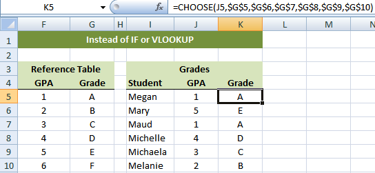Using the table above our CHOOSE formula in cell K5 is:

=CHOOSE(J5,G5,G6,G7,G8,G9,G10)

Or, if you’d used a VLOOKUP your formula would have been:

=VLOOKUP(J5, F$5$:G$10$,2)

Or, if you’d used a nested IF statement your formula would have been:

=IF(J5=1,”A”,IF(J5=2,”B”,IF(J5=3,”C”,IF(J5=4,”D”,IF(J5=5,”E”,”")))))

3. For a cool trick take a look at my CHOOSE and VLOOKUP example. All of a sudden you can make your VLOOKUP formulas look to the left!

Want more Excel Tips? Sign up for our newsletter below and receive weekly tips & tricks to your inbox, plus you’ll get our 100 Excel Tips & Tricks e-book.

Tagged as: lookup