Excel AVERAGE, AVERAGEIF and AVERAGEIFS

Let’s say that a baby learning to crawl is an analogy for learning the AVERAGE function in Excel.

Then learning the AVERAGEIF function is like learning to walk, and learning the AVERAGEIFS function is like learning to run.

So, lace up your shoes and get ready to run

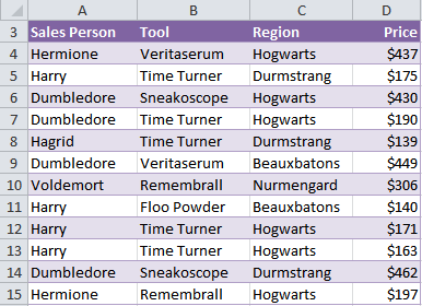
We’ll be using the table below in this tutorial. Inspired by my 5 year olds current obsession with the first Harry Potter movie.

Baby steps first:

Excel AVERAGE Function

=AVERAGE(your_data_range)

=AVERAGE(D4:D15)

=$271.58

As you can see, the Average function is fairly straight forward in that it simply averages a range of cells.

But there are some things you should know about how it works:

If one of the cells is blank it doesn’t include it in the number to average.

For example, there are 12 cells in our range D4:D15. So the AVERAGE function is actually summing the range of cells ($3,259), and then dividing them by 12 to get an average of $271.58.

But if cell D5 was blank it would sum the range of cells (and get $3,084) and divide them by 11 to get $280.36.

On the other hand, if cell D5 contained a zero it would still divide the sum by 12.

Excel AVERAGEIF Function

What if we wanted to get the average sales if the salesperson was Hermione?

That’s where the AVERAGEIF function comes into play. It allows you to average data in one range of cells where the data in another range matches a certain criteria.

The AVERAGEIF syntax is a bit different:

=AVERAGEIF(range, criteria, [average_range])

Where ‘range’ is the range containing your criteria, and [average_range] is the range of cells containing the values you want to average.

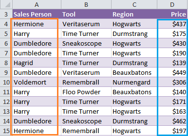
Let’s use the data below to find the average sales for Hermione.

Our formula would be:

=AVERAGEIF(A4:A15,”Hermione”,D4:D15)

=$317

In English;

=AVERAGE(referring to the range A4:A15, find Hermione, and average the values in the range D4:D15)

Note: the ranges of data must be the same size. In this example both refer to rows 4 to 15.

However, it wouldn’t work if one referred to rows 4 to 10 and the other referred to rows 4 to 15.

The limitation of the AVERAGEIF function is that you can only use one criterion.

AVERAGEIFS Function Syntax

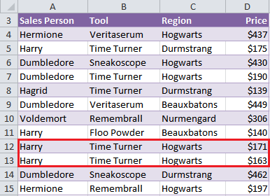
Whereas if you wanted to find the AVERAGE sales by ‘Harry’ of the product ‘Time Turner’ in the ‘Hogwarts’ region you’d need to use the AVERAGEIFS function.

=AVERAGEIFS(average_range, criteria_range1, criteria1, criteria_range2, criteria2,…)

Using our example data again our AVERAGEIFS function would be:

=AVERAGEIFS(D4:D15,A4:A15,”Harry”,B4:B15, “Time Turner”,C4:C15,”Hogwarts”)

=$167

Two rows match our criteria:

Download the Workbook

Download the sample file and take a look at some ways you can enhance your AVERAGEIF/AVERAGEIFS formulas using named ranges and data validation lists.

Enhancement 1: Named Ranges

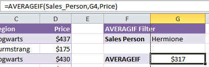
Notice in the formula bar how the first and last arguments of the syntax is ‘Sales_Person’ and ‘Price’ rather than a the cell ranges A4:A15 for Sales_Person and D4:D15 for Price?

This is called a named range and they make building your formulas quick and also easy to interpret later on.

Enhancement 2: Data Validation

In the AVERAGEIFS function I’ve also used named ranges. Plus I’ve used a data validation list or drop down list as they’re sometimes known as seen in action in the animation above.

The formula in cell G16 is:

=AVERAGEIFS(Price,Sales_Person,G11,Tool,G12,Region,G13)

This allows me to choose the criteria from the data validation lists in cells G11, G12 and G13 and the AVERAGEIFS formula will dynamically update to show the results for the new criteria.

Want to learn more tricks like this?

It’s techniques like this that I teach in my dashboard course to create reports that are interactive for the report recipient.

These features make your colleagues love you, because when you give them reports like this they are in control of getting the information they need quickly and easily.

And they save you time because you don’t have to create myriad of reports to cover every scenario.

It’s a win, win.

Click here to learn more about Excel Dashboard reports and how you can build interactive features into them.

Share This

Tweet

Please share this or leave a comment and I'll make sure you get a personal reply.