
In my previous Excel VLOOKUP formula tutorial I mentioned that there are two ways you can use a VLOOKUP but most people know one way or the other, and only a few know both.
As promised here’s the second way to use it, and I call it the Sorted List version as it relies on the data in the table you are referencing being sorted.
Note: If you haven’t read the first tutorial, then I recommend you first watch the video below from the beginning to get an understanding of how VLOOKUP works.
Excel VLOOKUP Formula Video Tutorial

Download the Workbook
Enter your email address below to download the sample workbook.
Excel VLOOKUP - Approximate Match on a Sorted List
First let’s set the scene:
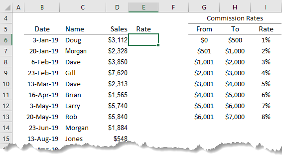
In the image below we want to lookup the Commission Rates table in cells G6:I13, and find the rate in column I based on the sales values in column D, and return the result to column E.
Excel VLOOKUP Function syntax:
=VLOOKUP(lookup_value, table_array, col_index_num, range_lookup)
And to translate it into English it would read:
=VLOOKUP(find this value, in that table, return the value in the nth column of the table, find an exact match if you can, but if not, find the next lowest match)
Note: with the Sorted List version we want Excel to find the next closest option in our table, i.e. an approximate match. To specify this we can leave the 'range_lookup' argument blank, or enter TRUE, or 1.
Excel VLOOKUP approximate match formula example:
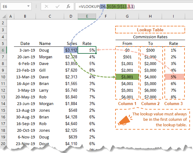
Remember we want Excel to find the Commission % Rate and enter it in cell E6, so in English our formula will read:
=VLOOKUP(find where the Sales amount $3,112, falls in the Commission Rates table G6:I13, return the value in column 3 of the table, if there isn't an exact match, find the next closest value)
And to enter it in our spreadsheet our formula in column E for the above example would be:
=VLOOKUP(D6,$G$6:$I$13,3, TRUE)
Let me clarify some points:
1) ‘find where Sales amount $3,112, falls in the Commission Rates table’ - Excel doesn’t actually take into consideration column H in our table. I have simply put it there to help understand the commission ranges. Excel is in fact looking for the exact amount $3,112 in our Commission Rates table, and when it can’t find it, it finds the next best lower amount and returns the value in column 3.
2) ‘Return the value in column 3 of the table’ is referring to the column number in the table G6:I13, not the column number of the spreadsheet. The information we want returned is the percentage rate, and it is in the third column of the Commission Rates table.
3) If we had consecutive duplicates in our Commission Rates table Excel will find the last instance of the value and return the result in column 3. For example, if instead of the amount $4001 in cell G11, you had $3001 again. Excel would return the value of 6% as it’s finding the last best match for our amount. The tip here is to remove any duplicates or you’ll end up with erroneous results.
4) Unlike the VLOOKUP Exact Match version of the formula, this version requires the list to be sorted in ascending order. Just like with duplicates explained above, if it’s not sorted you will end up with erroneous results.
You’ll notice in the formula bar above there are ‘$’ signs around the reference to the table. This is called an absolute reference and it allows us to copy the formula down column E without Excel dynamically updating the table range as we copy.
Want More?
Check out my previous tutorial for VLOOKUP Rules & Common Mistakes!


 Excel VLOOKUP Formulas Explained

Rod Leung
The tutorials are very helpful.
Mynda Treacy
Glad we can help, Rod 🙂
John Brewster
I have downloaded the Excel workbook, I haven’t practised on it as yet as I have not had the time but I will do and I look forward to practising on the workbook. I am waiting to go back to college and your tutorials will extend my skills from what I already know from the college, skills like Power Query which I find easier than complicated formulas like VBA. I will get back to you for a comment though.
Rick Chrysler
Very helpful
Diya Rao
Loved it. Well explained, way to go. I would like to know ore about data extraction for approximate matches using lookup function.
Mynda Treacy
Hi Diya,
Glad you found it useful.
If you have a specific example of your approximate match question please post it on our Excel forum along with your sample Excel file where we can help you further.
Kind regards,
Mynda
Manish Mandal
Thanks for sharing the use full with all of us,………
It is very helpful. it’s very helpful in office work & i can proud for it that i knows batter this other then my friends group, now i will be regular visitor of your site,,,,, Thanks Again !!!!!!!!
Mynda Treacy
Glad you found it helpful, Manish.
Cindy
Love your examples…make it easy for new users like me.
Q. I have a workbook with 27 tabs(sheets)I could use help with, please!
I have a tab for each letter of the alphabet that lists names, addresses, etc. and a column with conditional formatting returning a ‘Y’ if true. I would like the 27th tab (called “Mail List”) to be a list automatically created with the ‘Y’ value rows from the other 26 tabs.
At this point I’ve got one tab set up but it returns the ‘Y’ value row to the corresponding row on the “Mail List”(i.e. if the 9th row on tab “A” has the ‘Y’ value, it copies the info to the 9th row on the “Mail List”.) I need the “Mail List” to fill in from top to bottom no matter what line or tab it came from.
Is this possible? Is it easy enough for a new user like me?
Catalin Bombea
Hi Cindy,
Yes, of course it’s possible, if you get stucked in this process, let us know and we’ll help you. You can upload a sample workbook on our Help Desk.
Catalin
Phil Reinemann
In your clarification #2 you say “table H2:I9”. Did you mean table G3:I10 as specified in the formula “$G$3:$I$10”?
Also, I do like your use of the “so in English our formula will read” sections, along with the colorization “alignment” of the parts of the formula, carried from the Excel formula pop-up, to the English, to the actual formula. They help shed more light on what many people will find is lawyer-eze (any legal or financial document when read by a real person).
Good job!
Mynda Treacy
Cheers, Phil. Glad you like the English translations 🙂
Well spotted; H2:I9 should be G3:H10, I’ve fixed it now. Thanks for pointing it out.
Kind regards,
Mynda.
Jay Sadhu
hey Dear Mynda Treacy,,, Thanks alot for this wonderful contribution to my life ,it’s vry helpful in office work & i can proud for it that i knows batter this other then my office staff & my freinds group ,,,,now i will be regular visiter of your site,,,,,Again thanks alot Have fun !!!!!!!!
Mynda Treacy
You’re welcome, Jay 🙂
Patsiltri
I love this site, use it lots.
Q; I like to have a summary sheet that calculates totals from several tabs in the schedule. The tabs are named: one, two, three, etc. Is there a way to use the name of the tab in formulas like vlookup and sumif? That way I can put the tab names in the summary and use it as a reference in the summary tab formula.
Carlo Estopia
Hi Patsiltri,
Precisely, you can use indirect function to materialize this.
Try to download the workbook in this particular blog and look for the SUMIF part:
3D SUMIF Across Multiple Workbooks
An excerpt from the sheet, SUMIF: =SUMPRODUCT(SUMIF(INDIRECT(“‘”&tabs&”‘!A3:A8”),$A6,INDIRECT(“‘”&tabs&”‘!E3:E8”))) .
Note: the tab names are contained in the named range ‘tabs’.
However, I don’t know how you would like to do it in a VLookup. Although it’s still possible to use indirect function together
with a VLookup function but it doesn’t make any difference at all. You may want to use this syntax/formula in the same sheet of
the downloadable file above:
=VLOOKUP(A4,INDIRECT("'"&tabs&"'!A2:B2"),2,FALSE)Cheers,
CarloE
Enoch
Wow….this is new discovery for me.
Thanks
Mynda Treacy
Fantastic!
Dave
I need to create a vlookup (or “If” / “Or” statement) that only looks for values that are >229.0 or (but) 870 but less than 876.00. A sorting function.
Thanks
Carlo Estopia
Hi Dave,
I don’t think this can be done by a Vlookup function.
Cheers,
CarloE
sartaj
Thanks for sharing the usefull with all of us,………
It is very helpful.
Thanks once again.
Mynda Treacy
Thanks, Sartaj 🙂
Joseph Horling
Hi,
Just wanted to comment that your online training hub is really helping me in reviewing excel. Thanks so much for the simple explainations and the downloads to practice. And keeping it for free. Joe for Michigan.
Philip Treacy
Thanks. Glad you like it, Joseph 🙂
Brian Nyanzi
it is a good resource
Mynda Treacy
Cheers, Brian 🙂
taimoor
Best of luck dear. Your this addition is helpful to me. as my job is relating to such condition VLOOKUP
Mynda Treacy
Thanks, Taimoor.
Eskinder Haile
This is a good tutorial for those of us who want to understand Vlookup
Mynda Treacy
Thanks, Eskinder 🙂
Eric Juliana
Hopi bon,
Very good!!!!
Mynda Treacy
🙂 Cheers, Eric.
ASGHAR
I am a regular reader and as usual I find this article bearing much and useful information
Mynda Treacy
Thanks, Asghar 🙂
niyaz
good
Roy Lachica
This is such a good reference / resource for my office work which involve large data… thanks…
Mynda Treacy
Thanks Roy. Glad to help.
dtg
this site is fast
Fawaz
Finally i found it as a great method to learn excel here.
Thanks a lot to the organizers.
Craig Forrester
thanks, most useful to me
Andy G
great stuff. I think I understand vlookup now 🙂
roclafamilia
Helpful blog, bookmarked the website with hopes to read more!
hmm...?
thanks
Reg
This is such a great resource that you are providing
Philip Treacy
Thanks Reg. we really do hope people get a lot from our training. Spread the word 🙂