In this tutorial we’re going to explain how to use the Excel IF function (also known as IF Statement), and look at a couple of different applications for it.
With the IF statement you can tell Excel to perform different calculations depending on whether the answer to your question is true of false.
Watch the Video

Download Workbooks
Enter your email address below to download the sample workbook.

IF Formula Builder
Our IF Formula Builder does the hard work of creating IF formulas.
You just need to enter a few pieces of information, and the workbook creates the formula for you.
Excel IF Function Written Tutorial
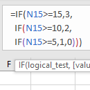
The function wizard in Excel describes the IF function as:
=IF(logical_test,value_if_true,value_if_false)
But let’s translate it into English and apply it to an example:
In the table below we want to calculate a commission in column G for each Builder based on the number of units in column D.
 |
We’ll say that for units over 5 we’ll pay 10% commission based on the Total $k figure in column F, and for units of 5 and under we’ll pay 5% commission.
Our IF formula for row 2 would read like this:
=IF(The number of units in cell D2 is >5,Then take the Total $k in cell F2 x 10%, but if it’s not > 5 then take the Total $k in cell F2 x 5%)
The actual formula we would enter into Cell G2 would be:
=IF(D2>5,F2*10%,F2*5%)
Remember; as the number of units in row 5 is not greater than 5 the formula would calculate a 5% commission.
Other Uses for IF
We don’t have to use the IF function to perform a calculation. We could use it to return a comment. If we take the previous example again, we could have asked Excel to put a note in the cell like ‘Pay 5%’ or ‘Pay 10%'. To do this our IF formula would look like this:
=IF(D2>5,"Pay 10%","Pay 5%")
Notice the difference between the two formulas are the inverted commas (") surrounding the results we want Excel to produce. These inverted commas tell Excel that the information between them is to be entered as text.
Below is a screen shot of how the formula looks in the Formula Bar and the result returned in column G.

Try Other Operators
Because the IF formula is based on logic, you can employ tests other than the greater than (>) operator used in the example above.
Other operators you could use are:
| = | Equal to |
| < | Less Than |
| <= | Less than or equal to |
| >= | Greater than or equal to* |
| <> | Less than or greater than |
*If we’d used this operator in our above example row 5 which had 5 units would have returned Pay 10%.
IF, AND, OR Together
Congratulations, you're ready to tackle IF functions with multiple conditions using the AND function and OR function. Check out our Excel IF AND OR tutorial next, and use the embedded Excel files to practice as you learn.
Or learn how to use the IFS Function to handle nested IFs with ease.


Anna
I am trying to create a formula that will compare data in 2 cells in different tabs. One tab has the information in a table with headers going across. The other tab has the headers going down column A like a list and the data is in column B. I need to match the headers data from the table going across to match the data from the headers in list form. For example: Tab 1 has 4 columns with data header is in row 1 going across, A1 = Apples, B1 = Oranges, C1 = Kiwi. With data being in the next row (A2, B2, C2).
Tab 2 has the list in different order going down, A1 = Kiwi, A2 = Apples, A3 = Oranges. with data in the next column (B)
Are you able to assist?
Mynda Treacy
Hi Anna,
This is a job for INDEX & MATCH. If you get stuck, please post your question on our Excel forum where you can also upload a sample file and we can help you further.
Mynda
Anirban Bhowal
Please repond about Excell formula for bellow :
1) If A4 = *17,750.00* then B4= 17,750.00 .
2) If A10= *-* and A11= *1,700.00* then B10= 0 & B11= 1,700.00 .
Mynda Treacy
Hi Anirban, Your question isn’t quite clear. please post your question on our Excel forum where you can also upload a sample file and we can help you further.
Jayden
Hi
Trying to find a formula to turn a cell to red if the time in one cell is 30 minutes after the time in another cell for example
lets say in A1 the time is 5:25 and the time in E12 is 6:00 I would want E12 to turn Red because its more then 30 minutes after time in A1
Thanks
Mynda Treacy
Hi Jayden,
You need conditional formatting for that. You can use this formula in the conditional formatting rule: =E1-A1>TIME(0,30,0)
If you get stuck please post your question on our Excel forum where you can also upload a sample file and we can help you further.
Mynda
Jayden
I’m trying to create a specific dropdown list whereby IE Column A is a dropdown list already containing certain data validations from another worksheet, and linking it to Column B which is another dropdown list where by if Column A= to Value1(on the list), it would display options ranging from “Option 1”, “Option 2”, “Option 3”. And if Column A= to Value 2, it would display options ranging from “Option 4″, Option 5”, and “Option 6″. Can anyone help me with this? :”
Jayden
Column B*** would display options ranging from “Option 1”, “Option 2”, and “Option 3”. And if Column A= to Value 2, Column B*** would display options ranging from “Option 4″, Option 5”, and “Option 6″. Can anyone help me with this? :”
Mynda Treacy
Hi Jayden,
I think you’re after a dependent data validation list. Here are some tutorials:
– Excel Dependent Data Validation
– Excel Dynamic Dependent Data Validation
If you get stuck please post your question on our Excel forum where you can also upload a sample file and we can help you further.
Mynda
CHE
Can you help me this for formula
IF C5 is equal to six amount of B5 multiply by 30%, IF C5 is equal to 5 amount of B5 multiply by 25%, IF C5 is equal to 4 amount of B5 multiply by 20%, IF C5 is equal to three amount of B5 multiply by 15% .
Catalin Bombea
Hi,
try:
=B5*INDEX({0.15, 0.2, 0.25, 0.3}, MATCH(C5,{3,4,5,6},0))
Daniel Doncovio
I’m trying to get a formula that will calculate in the following manner –
If Cell E10 = A then Calculate A20x I20
If Cell E10 = B then Calculate A20 x J20
If Cell E10 = C then calculate A20 x K20
Can you help me with this?
Philip Treacy
Hi Daniel,
Try this
=IF(E10=”A”, A20*I20, IF(E10=”B”, A20*J20, IF(E10=”C”, A20*K20)))
regards
Phil
Tori McC
I am attempting to create an If/Then rule in an Excel file. I have a column (C) that has a Yes/No drop down. I would like the next column (D) to assign a number (1 for yes, 0 for no) automatically. Is this possible? I cannot figure out the rules language to make it work. Thanks in advance for any help.
Mynda Treacy
Hi Tori,
Yes, it’s possible. In column D enter this formula and copy down (assuming the first row is 2):
Assuming there is always either Yes or No in column C.
Mynda
Emma
I have the raw attendance of my team in one tab and I created an IF statement to identify whether they are tardy or on time based on their scheduled time in (8 am PST).
N2 = actual log in
O2 = scheduled
=IF(N2>02,”Late”,”On Time”)
I created another sheet which will basically the dashboard. How to I lookup if an employee is on time or late with their name and dates as the criteria?
Mynda Treacy
Hi Emma,
It’s difficult to give you an answer without seeing the layout of your file. Please post your question on our Excel forum where you can also upload a sample file and we can help you further.
Mynda
Janet Branco
I am trying to create a formula to add a name in a column if two columns have specific information. IE, Column A reads, 0282 and Column C reads, D1, the Column D will be “Dena”. Can anyone help me?
Mynda Treacy
Hi Janet,
If that’s not what you meant, please post your question on our Excel forum where you can also upload a sample file and we can help you further.
Mynda
Sara
For my case,I have a cell which contains value till 1550, I need to amend 1 if the value shows 1 to 25, similarly if the value shows 50 to 100,I need to amend 2, like wise the formula needs to check until 1550,for each value the number should increase one each..and if it’s 1500 to 1550 it should come 62..so I couldn’t enter multiple ifs in single cell..so is there any way to make a formula simple. Instead of putting multiple ifs and AND,I just need a single formula..like the formula itself need to add 1 for each if
Philip Treacy
Hi Sara,
Please start a topic on the forum and attach your file. It’s really hard to visualise your data just from this description.
Regards
Phil
Shanell
I am unable to formulate this correctly : =IF(E11>100002000040000,E11*3/100)))
Please assist me. It answers to false.
Catalin Bombea
Hi Shanell,
You don’t have the value_if_false argument, you only put E11*3/100 for value_if_true:
=IF(E11>100002000040000,E11*3/100,”Replace with value needed if logical test returns false”)
The 100002000040000 value looks quite large, there may not be any value larger than that condition.
Carmen
If I want a cell to return a value of 50% if another cell is between 25-49 what would the formula be?
Catalin Bombea
Try this:
=IF(AND(A1>=25, A1<=49), 50%, 0)
Jeremy
If I have a month name (no date) in a cell *=(ex. A1) that changes and I want another cell to change to the next month (ex. A10), what formula do I use? So every time I change the name in A1, cell A10 will change to the name of the following month.
Mynda Treacy
Hi Jeremy,
You can convert the month name to the following month’s name with this formula:
=TEXT(DATE(2022,MONTH(DATEVALUE(A1&”1″))+1,1),”MMM”)
Mynda
Tanmay Newase
Using IF statement, apply discount of 2.50% for Particulars having price less than or equal to Rs. 3800/- and 5.00% for Products having price greater than Rs. 3800/-
Catalin Bombea
Discount% =IF(A1<=3800,2.5%,5%)
Flor Danica
Please help me with this in google sheet:
If the time difference between the two values in cells A1 and A2 is greater than 15 minutes and A1 falls outside of 12 midnight, then the cell will be highlighted.
Thank you very much!
Mynda Treacy
Hi Flor,
You need conditional formatting for this. If you get stuck, please post your question on our Excel forum where you can also upload a sample file and we can help you further.
Flor Danica
My formula in conditional formatting is =B1-A1>TIME(0,15,0) but for the example below…
Cell A1=(11:57:19 PM) – Cell B1 (12:23:51 AM)
its difference is 0:26:31 and It should be highlighted because it lasts longer than 15 minutes, but it wasn’t highlighted.
I don’t know what’s something wrong or lacking in my formula.
Mynda Treacy
Hi Flor,
Please post your question on our Excel forum where you can also upload a sample file and we can help you further.
Deidra Cooper
=IF(AND(A2:A9<=0,C2:C9<=0),"BLANK","CELLVALUE") – Using this formula….how do I get the data that is not blank to show? So what do I need to put in where "CELLVALUE" is? Thanks!
Mynda Treacy
Hi Deidra,
Enter the cell reference in place of “CELLVALUE”. e.g. If you want to return the data from cell A2 you’d write this:
=IF(AND(A2:A9<=0,C2:C9<=0),"BLANK",A2) Note that unlike text, cell references are written without the double quotes. If you want to return a range, then you have to tell Excel how you want to aggregate that range e.g. wrap it in SUM: =IF(AND(A2:A9<=0,C2:C9<=0),"BLANK",SUM(A2:A9)) Or if you have Microsoft 365 or Excel 2021, you can spill a range: =IF(AND(A2:A9<=0,C2:C9<=0),"BLANK",A2:A9) If you're still stuck please post your question on our Excel forum where you can also upload a sample file and we can help you further.
Mynda
johannes
im trying to find a formula like [ =if( D4>=$200,Discount 3%,no discount)
Mynda Treacy
Hi Johnnes,
If the value_if_true and value_if_false arguments are text, they should be wrapped in double quotes:
=IF(D4>=$200,”Discount 3%”,”no discount”)
Otherwise, your formula looks fine. If you’re still stuck please post your question on our Excel forum where you can also upload a sample file and we can help you further.
Mynda
Helen
Hi, I’m trying to create an if function allowing for VAT calculations.
I’ve got the formula to work for part of it but am stuck for the second part.
Where o16 is blank, return E16,
=IF($O16=””,$E16,xxxxx
for the second part I want it to work out where o16 contains an amount, perform the sum of o16 + R16. Any help would be really appreciated!
Mynda Treacy
Hi Helen,
You’re almost there:
You may need to play around with the absolute references as I’m not sure where you’re copying the formula.
Mynda
Helen
Thank you so much Mynda, I had been looking at is so long I couldn’t see for frustration!
Sankar
if Column No.1 is Yes
Column No.2 is Value represent in Colum No.3
Catalin Bombea
Hi Sankar, use this formula in C3:
=IF(AND(A1=”Yes”,B1=”Value”),True,False)
blakeaugust
=IF(C3>=10000),20% discount, “Donate”) please help me with this, thank you very much:)
Philip Treacy
Hi,
What are you trying to do with the IF?
What is the 20% discount being applied to?
Or do you just want the text 20% discount? If so, try this
=IF(C3>=10000, “20% discount”, “Donate”)
Regards
Phil
howard
Hi, I am stuck please help,
I am in VBA and the the code is below but if I remove the “a” in G10 or L10 then E12 must become “” (Blank)
Private Sub Worksheet_Change(ByVal Target As Range)
If Not Intersect(Target, Range(“G10:L10”)) Is Nothing Then
‘ MsgBox “It will Add a 0 to Cell E12 that you need to remove manually once you delete the (a)”
Range(“E12”).Value = 0
End If
End Sub
Mynda Treacy
Hi Howard,
This tutorial is for the spreadsheet IF function, not VBA. Please post your question on our Excel VBA forum where you can also upload a sample file and we can help you further.
Thanks,
Mynda
naso khan
ifcell(B2)>0 but cell(B2)=ifcell(B2)>600000 but cell(B2)=ifcell(B2)>1200000 but cell(B2)=ifcell(B2)>1800000 but cell(B2)=ifcell(B2)>2500000 but cell(B2)=<3500000,then company will charge you 17.2%+195000 money
Mynda Treacy
Hi Naso,
You should use a VLOOKUP formula on a sorted list rather than IF for this type of formula.
Mynda
Celina Gill
If O1 is <=1000, divide by K4. If results of O1/K4 is less than 50, return a blank cell. For the life of me I can not get the IF statement to get this result.
Mynda Treacy
Hi Celina,
Mynda
Nabeel
” Up to 100000 – 0%
Above 100000 to 200000 – 20%
Above 200000 – 30%”
How to solve above equation in excel
Mynda Treacy
Hi Nabeel,
For this you should use a VLOOKUP formula on a sorted list, not IF.
Mynda
Leslie
Losing my mind trying to recall the formula to highlight blank cells within a column, IF the date in another column exceeds 14days from the current date.
i.e. cells from J7 down, to be highlighted pink if the sum of the date in I7 down is greater than 14 days past the current date in cell J1 (which is a “TODAY” formula)
Mynda Treacy
Hi Leslie,
Please see this tutorial on conditional formatting formulas. If you’re still stuck please post your question on our Excel forum where you can also upload a sample file and we can help you further.
Mynda
Heidi
Is there a way to: turn Cell R12 red IF cells C12, D12, L12, M12, N12, P12, Q12 = N (for “no”). IF any of those cells have a “N” R12 should turn red.
Mynda Treacy
Hi Heidi,
Yes, you can use conditional formatting for this.
Mynda
lee
i need a formula when
every 1000dollar will be charge 1.5 dollar
Catalin Bombea
Try:
=RoundDown(A1/1000,0)*1.5
Kevin C
How would you enter and IF statement that displays the work “No” if an amount is less than or equal to zero and “Maybe” if the amount is greater than zero?
Mynda Treacy
Hi Kevin,
Mynda
Erika F
I don’t know how to explain what I want in short so here goes nothing.
Assuming today is the 15th of the month
I want collumn E to show PAID on a light green back-fill if collumn D has a value of 15 or less. Or UNPAID on a light orange back-fill if the value of collumn D is 16-31
Assuming today is the 1st of the month only cells valued at 1 in collumn D would display PAID in collumn E
Assuming today is the 31st ALL cells in collumn E should display PAID
I would like it to be irrelevant to month or year only relevant to day.
I have my bills set on auto pay and I’d like my budget spreadsheet to auto update PAID bills vs UNPAID based on what day it is. I have the day they are scheduled to pay listed in collumn D currently.
Mynda Treacy
Hi Erika, you need both an IF formula and conditional formatting. Please post your question and sample Excel file on our forum where we can help you further: https://www.myonlinetraininghub.com/excel-forum
Mia
Trying to figure out if cell C1 is equal to or greater to $100 then charge 10% or $15, which ever is greater, not to exceed $50.
Philip Treacy
Hi Mia,
It would be more efficient to use the LET function but you can do it this way
=IF(IF(C1>=100,IF(C1*0.1>15,C1*0.1,15),””)>50,50,IF(C1>=100,IF(C1*0.1>15,C1*0.1,15),””))
Regards
Phil
Mia
Hi Phil,
Thank you so much for your help. I will try it out. I’ve never used the LET function and will also attempt to learn this.
thanks again!
Mia
Philip Treacy
No worries
Ch sankararao
>200000 , AnD 200000 formula send me
Philip Treacy
Hi,
You need to supply more information. What is the result of the IF? What are the tests you want to perform?
Phil
Matilda
Hi – I am trying to create an excel document that will date stamp something when data in two different columns return something.
The data in each of these columns could reflect, upgrade, downgrade or no change.
Column a for example might reflect no change but column b might reflect upgrade or vs versa Column a and b could also reflect upgrade or downgrade.
Catalin Bombea
Hi Matilda,
A date stamp needs to be permanent i suppose? If you are looking for a formula, a date function will always recalculate and return today’s date, will not remain at the date when that change occurred.
Therefore, you might need a visual basic solution.
Can you please clarify and provide a sample file on our forum (create a new topic after you sign-up/in), for a better understanding of your situation?
Madhuri Narravula
Scenario is We have tasks which need to be completed with in the scheduled timelines however employees take extra days to finish the task.. existing excel has 3 dates …start time, end time and actual end date. In actual end date employee updates the date they completed the task. I need to get duration of days and if they have met or not met the deadline. Accordingly I have to find out the compliance percentages too. There is so much stuff in it and I need to get a dashboard out of this excel file on a MTD and Daily.
Please let me know if I provide u the excel can you help me on the outcome.
Mynda Treacy
Yes, it’s possible to do in Excel. Please post your question on our Excel forum where you can also upload a sample file and we can help you further.
Francis
Should I send my question and you fill for me
Mynda Treacy
No, just post it to the forum for anyone to answer for the quickest solution. Don’t address it to me specifically as I might not be able to look at it as quickly as someone else.
Md.Iqbal Hossain
IF A1 is < =75, then 4.19*A1
IF A1 is between 76-200, then 4.9*A1 +1*5.72(note:if A1=76; if A1=77 then it will be 2*5.72)
Mynda Treacy
Not sure how you can have two criteria for 77 i.e.
IF A1 is between 76-200, then 4.9*A1 +1*5.72
AND
If A1=77 then it will be 2*5.72
Please post your question and sample Excel file on our forum where we can help you further and our answers can also help others: https://www.myonlinetraininghub.com/excel-forum
Mynda
Krishna Wagle
Needs excel formula to calculate following:-
If value of C2 (in a cell) is greater than 150000, take value greater than 150000 but less than 200000 in C3(in a cell) but if value of C2 is less than or equal to 150000 than ignore it. Please enlighten by providing the formula in MS Excel.
Mynda Treacy
Hi Krishna,
You haven’t provided all the information, but you can start with this and modify as required:
If you get stuck please post your question on our Excel forum where you can also upload a sample file and we can help you further.
Mynda
Krishna Wagle
Thanks for replying. However, the formula while applying is shown as false. My question is follows:-
The value of C2 is Rs.240000. From the value of C2, amount exceeding Rs.150000 but less than Rs.200000 is to be taken in next cell (say cell C5) and if value of C2 is equal to or less than Rs.150000 (C2) take as zero.
Hope you will clarify and enlighten with formula for calculating the same.
Mynda Treacy
This is not clear “From the value of C2, amount exceeding Rs.150000 but less than Rs.200000 is to be taken in next cell”
Please post your question and sample Excel file on our forum where you can show us your desired result in an example and we can help you further: https://www.myonlinetraininghub.com/excel-forum
Krishna Wagle
Thanks. My question is that employees are submitting Income tax saving documents such as Rs.100000, Rs.134000, Rs. 200000, Rs.260000, etc. Exemption limit is Rs.150000 only irrespective of saving documents submitted by them under particular section. If employees submitted saving documents for Rs.120000, the whole amount is exempted as it is less than Rs.150000 but if employee submitted saving documents for Rs.210000 his exemption is limited to Rs.150000 as per Rules. However, saving documents beyond Rs.150000 subject to a maximum of Rs.50000 can be exempted under another section. As the employee submitted saving documents of Rs.210000, he can get additional exemption of Rs.50000 in another section and excess amount of Rs.10000 to be ignore.
My question is that an employee has submitted saving documents amounting to Rs.240000 and maximum amount of Rs.150000 is exempted in particular section and amount exceeding Rs. 150000 is to be exempted in another section subject to the limit of Rs.50000 only and rest amount to be ignore. However, if saving document submitted by employee is less than Rs.150000 the same to be ignore for exemption in another section. (If the value of C2 is greater than 150000 takes value greater than 150000 but less than 200000 in another cell and if value of C2 is less than or equal to 150000 ignore or takes zero).
Hope you will reply to my query.
Mynda Treacy
Please post your question in the forum and include your Excel file. It is much easier to understand an example file than try and follow paragraphs of text. Thanks for understanding.
Gulrez Rizvi
How to create report of inventory list of a particular commodity and date or a daily sales report of a flight by giving flight number and date , to obtain the ticket numbers with passenger details.
Mynda Treacy
Hi Gulrez, please post your question on our Excel forum where you can also upload a sample file and we can help you further.
Krista Stephan
Hello. I am trying to use my excel spreadsheet to identify when a date is out of compliance based on a category assigned. For instance tier 1 (g) requires a visit within 3 months of its last date (h) if > 3 months I need excel to identify that out of compliance but if (g) is tier 2, I need alert on (h) for non compliance > 6 months. Is that possible?
Catalin Bombea
Hi Krista,
Can you prepare a sample file with some examples? Will be much easier to help you.
Use our forum to create a new topic and upload the sample file.
Catalin
Candace
I need to do a formula that if there is a Y in column I then the following formula must apply 0.01*(AM4+AK4+AX4+AR4+M4) for column BC. If column I is blank then it should return a 0 in column BC.
Catalin Bombea
Try this in BC2:
=IF(LEN(I2)=0,0,0.01*(AM4+AK4+AX4+AR4+M4))
Makesense
Hello, please i want to convert a column of data from one range 0 – 50000 to another range 5 – 90. How do i go about it? I have tried to form a formula but haven’t been successful so far
Mynda Treacy
Not sure what you mean. Please post your question on our Excel forum where you can also upload a sample file and we can help you further.
Zahir Sabit
Very interested.
Mike
=EDATE(G10,(DATEDIF(G10,H10,”m”)+1)*1). This calculates the end date in terms of months and years. Can this string be used for showing “days” instead of months and years?
Many Thanks
Mynda Treacy
Hi Mike,
This formula returns a date. Perhaps if you provide some inputs for the dates in G10 and G10 and an example of the desired result we’ll better understand what you’re wanting to see and can help you further. Please post your question and sample Excel file on our forum: https://www.myonlinetraininghub.com/excel-forum
Mynda
wes
I have a simple formula needed but cannot figure it out. I need the column cell in G to turn red or green if it does not or does equal that value in column F.
Mynda Treacy
Hi Wes, you can use conditional formatting with formulas to do this. The formula will be something like:
=G2<>F2
No IF required because conditional formatting requires a TRUE/FALSE result. More in the tutorial linked to above.
Mynda
Rajesh Barman
“HIGH” if revenue is more than equal to Rs
1000 and “LOW” if revenue is less than 1000. how can do it?
Philip Treacy
Hi Rajesh,
Assuming you have your revenue value in cell A1 use this
= IF(A1 >= 1000, “High”, “Low”)
Regards
Phil
Tom
I have got this so that if B3 contains Pass the cell with the formular changes to 10:
If =value(IF(B3=”Pass”,”10″)
How can I get the same cell to change to 20 if B3 becomes Merit? (and then 30 if it becomes Distinction)
Mynda Treacy
Hi Tom,
Let’s say the value is in cell B3, the formula would be:
=IF(B3=”Pass”,10,IF(B3=”Merit”,20,IF(B3=30,”Distinction”)))
Mynda
Ben McFadden
Hi,
Formula I currently have is as follows;
=IF(B45<=50,450,450+((B45-50)*D45))
I still need the above but I also want to add to it that if B45 is left blank, a value of 0 is shown.
Thanks in advance!
Mynda Treacy
Hi Ben,
You need a nested IF formula:
=IF(B45=0,0,IF(B45<=50,450,450+((B45-50)*D45))) Mynda
Ben McFadden
Perfect! Thanks for your help!
IVA RANK
How can i make this formula continue from line 6 to line 57
=IF(G5+G6-E6>=480,480,G5+F6-E6)
Mynda Treacy
Copy and paste? Perhaps I’m not understanding what you mean. If so, please post your question on our Excel forum where you can also upload a sample file and we can help you further.
Maureen Lymer
I have been using this formula for years
‘=IF(OR(C3>140,D3>90),”Yes”,”No”)
but now they want to find C3>140 but less than 160
or D3 >90 but less than 100. Can’t seem to do the range bit.
Please help.
Mynda Treacy
Hi Maureen,
Try this:
Mynda
Imran
Hey,
Could help me with the problem?
Q1. Five different companies sold five different products by you. And gave you the commissions as 5%, 10%, 15%, 20%, 25%. Make the formula in excel sheet.
Catalin Bombea
Hi Imran,
We do our best to reply within 24 hours, but it’s not an instant service, sorry to disappoint you.
However, we do not answer school test questions and your question seems like it.
Just a tip: read comments below, you’ll find an INDEX MATCH solution.
John Lim
Hi all, can you help me on this
=IF(Q10=BW10,”PAID”,IF(BW10Q10,”OVERPAYMENT”)))
i want to add additional formula: incase the input value is 0.00 (zero) the result is Unpaid
Q10 = 10,000.00
BW10 where you input the amount
Mynda Treacy
Hi John,
Try:
Mynda
John Lim
thank you so much Ms. Mynda
KAREN WIGREN
I need to create a nested formula with the IF and SUM functions that will check the total number of hours worked in 1 week and is equal to zero If the cell should display nothing I want “”
Mynda Treacy
Hi Karen, It’s difficult to give you a solution without seeing the layout of your data. Please post your question and sample Excel file on our forum where we can help you further: https://www.myonlinetraininghub.com/excel-forum
KOLINI TAUILIILI
I want a formula to calculate If the customer brought 3 or more add-ons, then my answer is 15%, otherwise my answer is 0 or “” (Blank)
Mynda Treacy
Hi Kolini,
=IF(A1>2,15%,0) Assuming A1 contains the number of add-ons.
Mynda
AWAIS MAZHAR
=IF(F4=400000,F4*0.001)+IF(F4>400000,(F4-400000)*0.0015)+IF(F4>500000,(F4-500000)*0.004)
What formula function is that please anybody?
Philip Treacy
Hi,
Not sure what to say, it’s an IF formula and looks like it’s calculating something like a commission based on the value in F4.
Regards
Phil
AWAIS
THANKS,
Yes this formula is commission based. (D4= cell)
IF D4=400000 then commission D4 * 0.10%
Plus OVER 400000 LESS 500000 (D4-400000) * 0.15%
Plus OVER 500000 (D4-500000) * 0.40%
Please guide me.
Thanks
Philip Treacy
Hi Awais,
That commission structure seems odd. The first tier is only paid if D4 is exactly 400000?
Try this
Regards
Phil
AWAIS
Your Question:
That commission structure seems odd. The first tier is only paid if D4 is exactly 400000?
Answer: YES
But this formula not work.
=IF(D4>=400000,400000*0.001,0) + IF(D4>400000,IF(D4500000,(D4-500000)*0.004,0)
Philip Treacy
How exactly does it not work?
Please start a topic on the forum and attach your workbook so I can see what you are doing in your worksheet.
Regards
Phil
Jonathan
Hi, I am Jonathan, an excel novice.
I had the opportunity to learn it a long time ago, but I refused (that decision has come back to haunt me today).
My question is this, how do I return a column value to another column when the third column has another value.
For example. if a1=4 return b1 in c1
Catalin Bombea
Hi Jonathan,
In cell C1, use this: =IF(A1=4,B1,””)
David
I’ve input the formula: =DAYS(C1,A1) where these are dates. I’m wanting the total of days from when a document was submitted (A1) to when it was completed (C1). The formula works fine. However, our company is migrating to Google Sheets (hate it) when possible. Fine for the company, but not fine for us “superusers” that use excel for everything. My problem is the excel spreadsheet is stored on my Google Drive. When I go in to edit, all three columns setup with the above formula all show #NAME? instead of the days we seek. Plus, the formula line has this =xludf.DAYS(C1,A1).
If I delete the “xludf.” in the formula line and hit enter I get my days result. However, when I close the spreadsheet and come back a short while later. The =xludf.DAYS(C1,A1) is back again. Question, why is this happening and can I get a permanent fix?
Any help is appreciated. Thank you!
Mynda Treacy
Hi David,
Perhaps you can just change your formula to =C1-A1 as this returns the same result as =DAYS(C1,A1) and should be recognised by Google Sheets. Commiserations by the way. No more Excel will be very sad.
Mynda
David
I’ll try that thank you Mynda.
David
It worked great. Thanks again!
Schwann
I am really struggling with nesting formulas. add formulas to complete the table of hours used. in cell B17, create a nested formula with the IF and SUM functions that check if the total number of hours worked in week 1 (cells B9:F9) is equal to 0. if it is, the cell should display the total number of hours worked in week 1. copy the formula from cell B17 to fill the range B18:B20
Catalin Bombea
hi Schwann,
Please upload a sample file and describe where you need help, it’s hard to see a problem without a file.
Use our forum for upload.
Peter
Hi, Can you tell me formula for buy every 50000 and get 1 point, please…
Catalin Bombea
Hi Peter,
I think you should just divide the amount by 50.000:
=A1/50000
If A1 is 100.000 for example, the result will be 2. There may be fractional results, so you should use ROUNDUP, ROUNDDOWN or INT to remove the decimal places.
ACHIRE ANDREW EMMANUEL
Greetings Mynda Treacy. I want some help in developing an IF statement for the Schedule below. It is for our Local Service Tax for employment income deductions in Uganda.
Exceeding 100,000/= but not exceeding 200,000/= 5,000
Exceeding 200,000/= but not exceeding 300,000/= 10,000
Exceeding 300,000/= but not exceeding 400,000/= 20,000
Exceeding 400,000/= but not exceeding 200,000/= 30,000
Exceeding 500,000/= but not exceeding 200,000/= 40,000
Exceeding 600,000/= but not exceeding 200,000/= 60,000
Exceeding 700,000/= but not exceeding 200,000/= 70,000
Exceeding 800,000/= but not exceeding 200,000/= 80,000
Exceeding 900,000/= but not exceeding 200,000/= 90,000
Exceeding 1,000,000/= 100,000
Just to clarify, for instance in the first line, if the gross exceeds 100,000/= but does not exceed 200,000/=, then 5,000/= is the charge that they incur as tax. Waiting for your positive feedback. A full IF statement
Catalin Bombea
Hi Achire,
You can use a simple Index-Match combination:
=INDEX({0,5000,10000,20000,30000,40000, 50000,60000,70000,80000,90000 ,100000},MATCH(A1,{0,100001, 200001,300001,400001,500001 ,600001,700001,800001,900001 ,1000001},1))
You will have to play around with the limits: in this version, a number between 100001-200000 will return 5000.
pabitra kumar poddar
formula may be required
Priyant
=IF(I4>1000000,100000,(IF((I4900000),90000,(IF((I4800000),80000,(IF((I4700000),70000,(IF((I4600000),60000,(IF((I4500000),50000,(IF((I4400000),40000,(IF((I4300000),30000,(IF((I4200000),20000,(IF((I4100000),10000,0)))))))))))))))))))
I4 = in this cell you can put your salary
Cat Vaillancourt
URGENT
I’m looking to do a FAST input of my formula =IF(Oct!R2,Oct!P2,Oct!Q2), onto multiple worksheets
Such as
Tab 1 is titled “oct”,
Tab 2 through Tab 500, in the cell marked date,
I want to NOT have to go worksheet by worksheet to make changes the formula to reflect the correct line (example tab 3 – =IF(Oct!R3,Oct!P3,Oct!Q3), tab 4 =IF(Oct!R4,Oct!P,Oct!Q4) to pull from for each tab.
Is this possible?
Mynda Treacy
Hi Cat,
If you group the sheets first, then input the formula, it will insert it on each sheet relative to that sheet’s name. To group sheets, hold down SHIFT to select a range of contiguous sheets, or CTRL to select multiple non-contiguous sheets.
Mynda
Frank
I am trying to create a “shopping list” where someone would free text the item number and then have the price, UOM and vendor and some other fields autopopulate. Can this be done with this if/then formula? It is probably at least 500 items. I have all the info on excel file, i just need to make the shopping list
Mynda Treacy
Hi Frank,
Better to use VLOOKUP to lookup the item number and return the relevant price etc.
Mynda
Debasish Paul
I’ve a question , in excel left side column with two clause ” yes/no ” and in right side columns value with 1 1 1 1 that means sum 4 , but things is that , if i’m set a formula in a column left side clause is yes the sum sum should be done , if i’m select no the sum should be “0” .
if any formula is the then please help me.
Catalin Bombea
Try this one:
=IF(A1=”Yes”,SUM(C1:F1),0)
Joshua
Hi There,
I am looking for a formula which allows me to type 6M (which is a description of a shipping container meaning size 6 meter) in cell A1 and in cell A6 it brings up the transport price for a 6M container which is R3500.00.
Thank you 🙂
Mynda Treacy
Hi Joshua,
VLOOKUP would be better for this.
Mynda
Vinay Vyas
Hey,
I have put an extra space in the nested IF formula e.g. IF(G2<25, "10", IF(G2=30, "15", "0")) and got the answer.
Will it be considered wrong in my exam due to extra space instead i got the right answer?
Please clarify!!
Philip Treacy
Hi,
Spaces in a formula like this are irrelevant, so no this should not be considered wrong.
Regards
Phil
Vinay Vyas
Thanks for your reply Phil, I have one more doubt :
The question in the exam that was like: We have to allot grade to the student on the basis of hours. If hours are less then 25 then grade 10, if hours are equal to 25 than grade 15, if hours are equal to 30 than grade 20 and if hours are equal to 40 than grade 30. I used the formula : IF(G2<25, "10", IF(G2=25, "15", IF(G2=30, "20", IF(G2=40, "30", "0")))) .
My doubt is that, there wasn't any false condition that was given so I put "0" in the formula {I solved in this way because I couldn't remember another way at that time} because all the entries in the question were among above-given conditions. So in spite of getting the right answers for all the entries will it be considered wrong?
Some are saying there will come 3 if, some are saying 4 if and some are saying this way. So please clear the confusion.
Catalin Bombea
Hi Vinay,
It does not make much sense, what if a student has 27 hours? Will receive a zero and this is wrong, from 25 up to 30 it should receive 20 as the grade.
Try this, will take care of intermediate values as well:
=INDEX({10,15,20,30},MATCH(A1,{0,25,30,40},1))
Robert Paterick
How to move text from cell 1in sheet 1 to sheet 2 in cells 1,2, etc.sucessifly using vba code.
Catalin Bombea
Hi Robert,
Can you clarify? Is it the same entire cell that needs to be duplicated in multiple sheets? Or you need to split the text (in this case- which are the criteria/delimiters for splitting)?
Waqas Munir
Hello
if cell A1 have any text then d1 should get 2000 and if a1 and b1 both have some text then at the same time cell d1 should be filled with 4000
and if a1 is empty then b1 will also b empty in this case d1 should empty
if a1 have some text and b1 is empty then d1 should get 2000 i need a formula to resolve this query.
Philip Treacy
Hi Waqas,
Try this
Regards
Phil
Waqas Munir
Thank you so much Philip Treacy. Your given formula is working and problem is resolved.
In future if c1 also have some text then answer should be 6000,
i will be thankful if you guide for third situation.
Thanks for your cooperation.
Best Regards
Waqas Munir
Philip Treacy
Hi Waqas,
If there’s a value in C1, how does that work with possible values in A1 and B1 e.g.
Regards
Phil
Catalin Bombea
Try:
Waqas Munir
Hello Phil & Catalin – Sorry for late reply on this and the formula for C1 is not working.
Condition is that= if c1 have value then a1 and b1 will not be empty and a1 b1 also contains some text.
now I facing another problem which i have to resolve.
=IF(A1″”,IF(B1″”,4000,2000),IF(C1″”,6000,””)) after entering it i face an error.
please add one more condtion for A1 with this upper mention formula.
if A1 have specific text that is A1=2stops then answer 1000 and in case any other text answer 200
=IF(A1″”,A=”2Stops”,IF(B1″”,4000,2000,1000),IF(C1″”,6000,””))
please guide me the right formula as i mention the condition.
A1 B1 C1 Answer Cell
Any Text 2000
Any Text Any Text 4000
Any Text Any Text Any Text 6000
2Stops 1000
in last case A1 have just text B1 C1 will empty.
please guide me on formula for upper mention conditions.
Thanks in advance for your help.
Regards
Waqas Munir
Catalin Bombea
Hi Munir,
Please use our forum to upload a sample file with a few manual expected results, it’s hard to follow your instructions, a file with examples will be better hopefully.
NEIL
=IF(B5=”P”,P5*0.1+P5),IF(B5=”C”,P5*0.2+P5)
HOW TO MAKE THIS FOMULA CORRECT
Philip Treacy
Hi Neil,
Try this
=IF(B5=”P”,P5*0.1+P5,IF(B5=”C”,P5*0.2+P5,0))
Regards
Phil
ernest
i need faster and easier way to do my analysis as I don’t have much idea in vlook up and ifs.
Philip Treacy
Hi Ernest,
Not sure what to say. Learning things like VLOOKUP and IF is the way to do your analysis quicker. there are no shortcuts, you’ll just have to put in the time.
Phil
James Guy
Can a dashboard be created for online stock trading. Taking a course and would love to track using excel 2013, thanks. Oh, you are awesome. I’m looking forward for your teachings.
Catalin Bombea
Hi James,
Generally speaking, a dashboard can be created for anything, as long as you have data for that.
I guess it’s not just a dashboard you’re interested in, you might think about getting data too.
You can find info here for collecting live data.
Suth
=Ncb(0,0,P5,R5,C8,C8,1)
What formula function is that please anybody?
Catalin Bombea
Hi Suth,
That does not look like an excel formula, looks more like a custom UDF (user defined function, built in Visual Basic).
Cheers,
Mohamed Moqdad
Excellent Job.
Thanks a ton..
karabo
IF(B2>R1000,5%,10%)
steve
How do I make a row turn green if Column N is greater than Column M, but do nothing if Col M is greater than Col N?
And how do I make a row turn yellow if the text in Col B is made red using a conditional format?
Thank you
Mynda Treacy
Hi Steve,
You need conditional formatting for this. Have a go and if you get stuck please post your question on our Excel forum where you can upload your Excel sample file and we can help you further.
Mynda
Levi
I have this formula entered in, it does exactly what i want.
=IF((AND(C10>C9)), (G9+750), (G9))
But if C10 is blank I want this cell blank as well…
Please help, Thanks!!
Catalin Bombea
Try this:
=IF(C10=””,””,IF(C10>C9, G9+750, G9)) (Your AND function is redundant, there is only one condition)
JoKN
Yes, you are right, it does have a typo, my apologies.
=SUMIFS(A1:A3,(B1:B3),”>0″)
Mynda Treacy
Which yields the same results as the SUMIF formula Phil provided you:
This:
And this:
Do exactly the same thing. You don’t need SUMIFS because you only have one criteria, so SUMIF will suffice.
Mynda
JoKN
Thank you for your speedy reply.
I tried your formula but it was still returning an error. Perhaps this is because I am using Excel 2007?
I tweaked it a bit and found the solution
=SUMIFS(A1:A3),(B1:B3),”>0″
Thank you once again for your invaluable help in solving this for me!
Mynda Treacy
That formula must have a typo in it, because that’s not going to work as is.
JoKN
Hi,
I’m compiling a spreadsheet to keep track of payments made. There are 2 columns, one with the amount to be paid and the other with the date that the payment was made.
How do I make a formula that will keep a total of all that has been paid? I want the formula to only add the amounts that have a date entered in the column next to them.
Thanks
Philip Treacy
Hi,
If your payment amounts are in Col A and your dates are in Col B try this
=SUMIF(B1:B3,”>0″,A1:A3)
Regards
Phil
Susan
my formula is great and works for what I want, but if there is nothing in the cells, it still shows KPI met. Where the previous cell is blank, can I get it to realize that and stay blank itself?
formula is =IF(E2<=72,"KPI Met")
Once I've put the formula in the cell, it states KPI met although the preceding cell is blank. Any ideas?
Many thanks
Catalin Bombea
Hi Susan,
Try:
=IF(AND(E2<=72,F1<>“”),”KPI Met”,””)
Sam
What will be the function for all the cells to be replaced with P
Mynda Treacy
If you just want to replace everything with P you can select the cells and type in P then press CTRL+ENTER.
Sam
I want a function in excel where when I enter “A” as absent in respective Cells for a month then other cells are marked as “P”.
Mynda Treacy
Hi Sam,
Something like this:
Where cell B2 contains ‘A’ for absent.
Mynda
Craig
Guys, I need your help. I am creating a spreadsheet to calculate times, but I only wants excel to display the results if the HH:MM is less than 00:00. So in other words I only want the -00:00 times to be shown. I also want the negative result to shown with green font. Any brave soul wants to give this a try?
Philip Treacy
Hi Craig,
You can’t have negative time. Maybe if you open a topic on the forum and supply your workbook + data we might be able to figure something out.
Regards
Phil
Imelda Sanchez
Good Morning,
I have a list of Salaries and they vary from salary to hourly, i would like to specify Hourly or Salary on another column is the if function the appropriate function i should be using?
Mynda Treacy
Hi Imelda,
Yes, you could use IF for this assuming there is some way to tell the difference between hourly pay and salary pay.
Mynda
Dean
Hello,
I have written a spread sheet for horse racing,
I would like to remove an amount of percentage from the winning bets (Commision) but not the losing bets,
The amount to be removed (%) is in a seperate column,
G5 is either a win amount say 2/1 showing as 2 or a lost bet showing as -1
I5 is the percentage to be removed =SUM(J5*H5) stake times by percentage to be removed
K5 is the column I need the formula in to show the total after % removed =SUM(J5-I5*G5) (win) or lossed stake in full from column J5 (Stake amount)
Thank you
Kind Regards
Dean
Mynda Treacy
Hi Dean,
There is information missing from your question e.g. what is in cell J5, and it’s difficult to visualize the contents of all of the cells mentioned. Please post your question in our Excel forum where you can upload your sample Excel file and we can help you further.
Mynda
Yeswanth
How to calculate it in excel?
Rs.100 Upto 20 Box, Above 20 Box – Rs.5/- Per Box
Catalin Bombea
Hi Yeswanth,
Try this one:
=IF(A1<=20,100, 5)
Ashley
Is it possible to write a formula stating if a cell is greater than 500 then multiply everything over 500 by .05?
Catalin Bombea
Sure, why not?
In the next column, use this:
=IF(A1>500,(A1-500)*0.05,0)
Sandra
Hello
I want a formula that returns a value from a cell not the word true or false.
Cell a =Ice so I want Cell C to equal the value typed in Cell D
I have this but I get the word false instead of the number 12 that is typed in Cell D2
=IF(A2=”Ice”, C2=”D2″,IF(A2=”Candy”,C2=”D4″,IF(A2= “Pop”,C2=”D5″))))
Catalin Bombea
Hi Sandra,
The formula should be located in cell C2, you cannot choose the destination of the result in the formula:
=IF(A2="Ice", D2,IF(A2="Candy",D4,IF(A2= "Pop",D5,"Other Case")))
Chad
Please Help! I am trying to write a formula for calculating overtime in payroll. Basically if any value in column A is 40 or under it remains. If it is over 40, then in column B it calculates the difference from 40 and leaves 40 in column A.
Thanks a Million!!!
Catalin Bombea
Hi Chad,
Sounds like a simple problem, try this in cell B1, copy it down as needed:
=IF(A1<=40,0,A1-40)
Chad
Thanks for the quick reply. The formula works but leaves the original number that is over 40 in column A. Can you let me know how to reduce the number to 40 and have the difference in column B. For instance employee X has 56 hours in column A, it should change column A to 40 and B to 16. Thanks for all your help!!
Philip Treacy
Hi Chad,
You can’t do that. A function will only return its result into the cell its called from. So a function in B1 will put a result in B1, it cant change the value of A1.
You could take the values in A, have the worked time (up to 40 hours) in B and then have the overtime in C?
Regards
Phil
Rundull
Please help me resolve this issue
If A1=A or B then B1=1 else B1=2
Thanks!
Philip Treacy
Hi Rundull,
Put this in B1
Regards
Phil
yogaraj
Dear Experts,
Needed Help!
I have listed 100 color in Cell A and 100 color in Cell B for double color cloth.(Ex:- Red,Blue)
when i select cell A color and Cell B color it will be visible cell C.(Red/Blue)
if i did not select in Cell B,the cell A color only visible in cell C.the cell B value don’t visible cell C.(Ex:-Red).
How to manage this.? i have another one query if does not select cell B it will be auto hide without Macros?
Thanks,
Mynda Treacy
Hi Yogaraj,
Please post your question on our Excel forum with a sample Excel file so we can see what you are trying to achieve. Please also clarify what you mean by ‘select’; do you mean click on a cell with your mouse, reference a cell in a formula or something else?
Thanks,
Mynda
Sandie
I am having a problem with the IF formula. Will you please help me with this problem.
Create a formula using the IF function and structured references to determine the correct amount paid based on the following criteria:
If the Repeat? value is “Yes”, calculate the amount paid by subtracting 5 from the Fee.
Otherwise, the amount paid is the Fee value.
How would I type this out using the IF Formula?
Catalin Bombea
Hi Sandie,
Should look like this:
=IF(A1=”Yes”,B1-5,B1) or: =B1-IF(A1=”Yes”,5,0) (they will always give the same result)
If you want to apply the formula on a range that has more than 1 cell, it’s a different case, you should use:
=SUM(IF(A1:A7=”Yes”,B1:B7-5,B1:B7)) (confirmed with CSE, it’s an array formula)
Syed Raiyan Karim
It is very useful for self training
Mynda Treacy
Glad we could help, Syed.
Jimmy Ramirez
Hi, I just need an explanation about the IF logic that I saw. It shows like this;
=IF(ISBLANK($Z137),””,IF((INT($Z137)-$B137)<=IF($AC137="MIM",9,IF(OR($AC137="SGMA",$AC137="NGMA"),4,2)),"HIT","MISS"))
Can you please explain it one argument at a time?
Mynda Treacy
Hi Jimmy,
I’ll break your formula down into 3 parts. In English it reads:
1. [IF(ISBLANK($Z137),””] IF Z137 is blank then return nothing and stop there.
2. [IF((INT($Z137)-$B137)<=] Otherwise test if the integer of cell Z137 minus B137 is less than or equal to the result of the next IF. 3. [IF($AC137="MIM",9,IF(OR($AC137="SGMA",$AC137="NGMA"),4,2))] IF AC137 contains the text MIM, then return 9, otherwise IF AC137 contains the text SGMA OR NGMA then return 4, otherwise return 2. If part 2 compared to part 3 is true then return "HIT", otherwise return "MISS". Mynda
marco
=if(a1=22:00,b1,””) dos not working any help
Mynda Treacy
Hi Marco,
I suspect that 22:00 is either text or an actual time serial number.
For text try:
For time stamps try:
Kind regards,
Mynda
sarathy
is there any formula to get the gross value when added salary and bonus.
salary $k Bonus $k Gross $k
138 nill 138+nil=138
Catalin Bombea
Hi Sarathy,
What nil is? A percentage, a bonus amount? It does not look like an excel problem, more like basic math.
If it’s a percentage (I assume you can make the difference yourself if it was an amount), try Gross/(1+Percent), where percent should have values like 10%, 30%, not 10, or 30.
Ali
=IF(OR(K19>1,K19<J19,"Partial",IF(K19=J19,"Paid","Oustanding"))
WHAT IS WRONG IN THIS FORMULA
Mynda Treacy
Try:
1234
find two mistake
=If(D5>=100,if(A4<=10,"100"),TRUE)
Mynda Treacy
Your question isn’t clear, but if you want both logical tests to be true then use AND like this:
Mynda
Feleti Wolfgramm
“This is very useful tips and how you present your the formulas are easy to follow. Keep up the good work.”
Feleti
Mynda Treacy
Thanks, Feleti! Glad you found it helpful 🙂
Olusegun Osewa
Hi,
I am really stuck with this IF Statement: =IF(F5=(I5+J5),”TRUE”,”FALSE”). It is not giving the right results. Please help.
Philip Treacy
Hi,
You don’t say what error you are receiving, when I type this out it works ok for me
I did notice that in your comment you had TRUE and FALSE encased in slanted/curly quotes ” but they should be in straight quotes
if you want to use strings (text).
But neither TRUE nor FALSE actually need to be in quotes, you could just write it like this
Regards
Phil
Amy
HELP!!!!
We use google sheets for our time sheets and I am sure I am over thinking this, but I don’t have time to waste. So here goes….
Let’s say Employee A works 56 hours in one week. I need a formula that would take the total hours worked and subtract anything over 40 hours. I have the current formula to subtract the OT which is =IF(AD1>40, AD1-40, ” “) and that works great to take the hours over 40 and put them in that column and then calculates the OT pay. So I need to add a formula that does something similar.
So, something that does IF CELL “X” IS OVER 40 THEN IT TAKES THE NUMBER OVER 40 AWAY AND LEAVES 40 AND IF IT IS LOWER THAN 40 THEN IT JUST LEAVES THE NUMBER.
Hope that made any sense!
Mynda Treacy
Hi Amy,
Try:
Mynda
SABIN GEORGE
HI,
I AM ENTERING SOME COMPANY INFORMATION ON EXCEL SHEET LIKE COMPANY NAME, PHONE NUMBER, FAX NUMBER ETC. IF I REPEAT THE COMPANY NAME THERE IS ANY POSSIBILITY OR EQUATION THE PHONE NUMBER AND FAX NUMBER COMES AUTOMATICALLY?
Mynda Treacy
Hi Sabin,
You can use a VLOOKUP formula to lookup a list of items and return corresponding details like phone number etc. Here is a VLOOKUP tutorial.
Mynda
JJ
Hi. On Worksheet 1, if the response in Column D2:D73 is, of the various options available, “Cash”, then I’d like the corresponding Columns F and G in the same row darkened. How might I do that? Thank you.
Catalin Bombea
Hi,
You should use conditional formatting for this.
Select those 2 columns: F2:F73 and G2:G73, then add a conditional formatting rule based on a formula: =$D2=”Cash”
Choose any format you wish for this rule, cell interir color, borders, font color.
See this article to see how to use conditional formating.
Catalin
Kirk Patrick
I am looking for a formula that will do the following;
Well, I have a workbook with TWO sheets.
Sheet ONE has a template that calculates data, depending on some primary figure entered in a certain cell. These figures are distributed through a list of names in the same sheet. What I want is that, when these figures get calculated, they should be relayed in sheet TWO that contains the same names in the same order….and because we have different figures for different values entered in the primary cell, that means I’ll need to have these distributions relayed in different columns of sheet TWO as different values are entered in the primary cell of sheet ONE. Help? Maybe I could get you a copy of the document and understand it please.
Mynda Treacy
Hi Kirk,
Please post your question and sample Excel file on our Excel Forum where we can help you further.
Cheers,
Mynda
Diane
Hello – I’m stuck on an “IF” formula, can anyone help.
The question is: If the Repeat? value is “YES”, calculate the amount paid by subtracting 5 from the Fee, otherwise, the amount paid is the Fee value.
Repeat (F4) Fee (G4)
I had =IF (F4=”YES”,G4-5) My problem is, keeping the “NO” fee the same? What am I missing in the formula? Any help would be appreciated. Thanks
Catalin Bombea
Hi Diane,
IF function has 3 arguments: first is the logical test(F4=”YES”), the second is the value for a true logical test (G4-5), the third argument is the value if logical test is false, this is also the argument you missed.
It should be: =IF(F4=”YES”,G4-5,G4)
Diane
Hello Catalin,
Is that the only possible way of writing it? I turned in the assignment in Cengage with G4 on the end of the formula and it was kicked back saying the formula was not correct? So, I thought maybe I had the G4 wrong? Thanks, Diane
Catalin Bombea
Type again the double quotes, most probably the ones you copy pasted are different than the ones used in excel. Or type the entire formula again manually, there is no reason not to work, other than double quotes.
Diane
Hello again,
I have one more that was kicked back, maybe you can help with it too. Using the DSUM
The question is: Use the entire Student table including the heading row H3, use the amount paid header as the field argument, use the range J5:J6.
I have the formula =DSUM(Student[#ALL],H3,J5:J6
L.E.
Let me re-write the above question.
Use the entire Students table including the header row, use the amount paid header in cell H3 as the field argument, use the range J5:J6 as the criteria.
I had – =DSUM(Students[#ALL],H3,J5:J6 – which was incorrect
Catalin Bombea
Hi Diane,
Can you please upload a sample file on our forum? It will be a lot easier to help you. Create a new topic and add a sample file, we will gladly help you.
Cheers
Catalin
Karla
Hello I need help, to say if AD1 is greater than zero and AG1=coaching then take AE1 and put in AD25 and in the end I want to sum all items AE1throughAE24.
Mynda Treacy
Hi Karla,
I’m mot sure what you mean by “take AE1 and put in AD25″.
I’ll assume your formula is in AE1:
=IF(AND(AD1>0,AG1=”coaching”),AD25,0)
Mynda
Karla
Thank You Mynda, it works. I gave you the wrong columns yet I made it work. Here is the formula
=IF(AND(AE1>0,AH1=”coaching”),AE2,0)
Now my next step is if AE is greater than 0 and AH equals coaching then put it in cell AD 25 but I want to do this with all the rows so at the end I have a sum amount (total amount in AD25) of all rows that were greater than 0, and were labeled coaching. I hope this makes sense?
Mynda Treacy
Hi Karla,
You need SUMIFS for that. You haven’t said what column you want to SUM so I can’t give you a formula, but you can learn how to use SUMIFS here.
Mynda
nichelle
Can you please explain this equation for me?
=IF(F6=””,””,WORKDAY(F6,ROUND(Gates!$B$2,0)))
Mynda Treacy
Hi Nichelle,
In English your formula reads:
IF F6 is blank/empty, then return a blank, otherwise return the date that is +/- the number of working days in cell B2 rounded up/down to the nearest whole number.
Working days exclude Saturday and Sunday.
Mynda
Elinor
good day!
please help me find a formula for this; in C1:G1,or more columns to be added, are the spare parts of a car, and on B2:down are dates, and on C2:G10, or more columns and rows to be added, are amount of spare parts.
the problem is,
on sheet2, A2 down are dates, and on B2 down are the spare parts with amounts. for example if on sheet1 there is amount on C2, then on sheet2 B2 it will copy C1 on sheet1. and if there is amount on G3 on sheet1, then on sheet2 B3, it woll copy G1 on sheet1. what i mean is if there is amount on a certain spare part then it will copy or specify what is that spare part.
thank you and God Bless!!
Mynda Treacy
Hi Elinor,
Thanks for your question.
Unfortunately, it’s difficult to visualise your example. Can you please post your question on our Excel Forum and upload a sample Excel file so we can help you further.
Mynda
Thomas
I am looking for a Formula to track a players number of goals scored.
For instance Player A has 10 goals this season and scores 2 goals tonight.
The data query will update to 12 goals.
If the cell the goals are in is A1 I would want the changed data to show “+2” in B1 to reflect the data increase in A1.
Mynda Treacy
Hi Thomas,
I’m not sure what form this “The data query will update to 12 goals.” is in so it’s difficult to give you a solution, but you can certainly track change from one week to the next but you need to keep that data in separate cells.
It would help if you can post your question on our Excel forum with a sample Excel file containing your data and we can give you a specific solution.
Cheers,
Mynda
MOHAMMAD AHSAN HABIB
Good evening I need some help please. I need to formula ( Blue card value=100 taka)
if purchase 5000 he get 1 blue card,
if purchase 15000 he gets 3 blue card,
if purchase 30000 he gets 6 blue card and 1 blue bonus card.
if purchase 50000 he gets 10 blue card and 2 blue bonus card,
if purchase 100000 he gets 20 blue card and 5 blue bonus card
if purchase 150,000 he gets 15 Green card ( green card value=250)
if purchase 200,000 he gets 20 Green card and 1 Green bonus card
if purchase 300,000 he gets 30 Green card and 2 Green bonus card
if purchase 500,000 he gets 50 Green card and 10 Green bonus card
please helf
Catalin Bombea
Hi Mohammad,
Try this one:
=INDEX({"-","1 blue card","3 blue cards","6 blue cards + 1 bonus blue card","10 blue cards + 2 bonus blue card","20 blue cards + 5 bonus blue card","15 green cards","20 green cards + 1 bonus green card","30 green cards + 2 bonus green card","50 green cards + 10 bonus green card"},MATCH(A13,{0,5000,15000,30000,50000,100000,150000,200000,300000,500000},1))Leslie
Good evening I need some help please. I need to select information from 2 different cells to give a value in a 3rd cell,
The example being of cell AV73=1 and if cell AV87=0.8 then the cell AV75 should have an answer of 1. Similarly if cell AV73=1 and if cell AV87=1.1 then the cell AV75 should have an answer of 1.5. Similarly if cell AV73=2 and if cell AV87=0.8 then the cell AV75 should have an answer of 1.2. and finally if cell AV73=2 and if cell AV87=1.1 then the cell AV75 should have an answer of 1.4.
I hope that this makes sense. You help will be most welcome.
Catalin Bombea
Try this in AV75:
=IF(AND(AV73=1,AV87=0.8),1,IF(AND(AV73=1,AV87=1.1),1.5,IF(AND(AV73=2,AV87=0.8),1.2,IF(AND(AV73=2,AV87=1.1),1.4,”Other”))))
Leslie
Thank you so very much Catalin. I really appreciate it. As I am doing a research paper I would like to reference you by name and title and job title. Can you provide this. Thank you once again. It works perfectly. Am truly grateful.
Catalin Bombea
Hi Leslie, Glad to hear that it works!
I think you should reference the creator of this article, Mynda Treacy, Co-Founder of MyOnlineTrainingHub, I am the Excel Support Guru on this website.
Regards,
Catalin Bombea
Kevin Lim
=IF(H7=””,””,DATE(RIGHT(H7,4),MID(H7,4,2),LEFT(H7,2)))
What does above formula do?
Mynda Treacy
Hi Kevin,
The formula is converting text dates into proper Excel date formats. In English the formula reads:
If cell H7 is blank then return a blank, otherwise return a date made up of the 4 right-hand characters, the middle 2 starting at the 4th character and the left 2.
Mynda
Kaiser
Thank you so much for sharing. I was trying another problem similar to your issue, how can I write the formula for such problem:
This is your formula =IF(D2>5,”Pay 10%”,”Pay 5%”) for two options, but I was trying to put another formula which is not working, like: = IF(A2100001,”MD”). Can we get 3 options in 1 formula. Actually I want the selection of HORB, DMD, MD depending on the value provided in A2. Is this possible? Please advise.
Catalin Bombea
Can you provide the values range for HORB, DMD, MD?
Like:
HORB: from 1 to 4
DMD: from 5 to 10
MD: >= 11
Is the result depending on multiple cells evaluation, not just D2 (or A2, you mentioned more than 1 cell) from your example?
Kate
Hello!
I guess my question goes a little more in depth! I have a multi spreadsheet document and I am trying to do a If/than type of formula with many brackets (6). The first one works accurately, but when add the last 5, I believe it has something to do with the way I am adding the brackets around the continuing formula…Here is what I am attempting…
=IF(‘4 – Lead Line Equ.’!A3=1,”7″,(‘4 – Lead Line Equ.’!A3=2,”5″),[‘4 – Lead Line Equ.’!A3=3,”4″],[‘4 – Lead Line Equ.’!A3=4,”3″],[‘4 – Lead Line Equ.’!A3=5,”2″],[‘4 – Lead Line Equ.’!A3=6,”1″])
Mynda Treacy
Hi Kate,
You need this tutorial : nested IF formulas
If you get stuck please post your question on our Excel forum with your sample Excel file and we can help you further.
Mynda
Ashley Dickieson
Great and thorough explanation!
I can’t seem to figure out if this formula could work with what I want to do.
If column A in my spreadsheet has a certain date, I want column B to have a status.
For example,
If the date in column A is less than 9 months ago, column B should say current.
If the date is 9-11 months ago, I want B to say 9-11 months. And so on for 1yr + etc
Any suggestions ?
Mynda Treacy
Hi Ashley,
It’s best to use a VLOOKUP on a sorted list for this.
If you get stuck please post your question on our Excel Forum with your sample Excel file.
Mynda
schnaider
Can some one help on this every time I do it it’s never returning the values for those >400 and values > to 500.
I wanted to do a payroll where someone gets 40% if they can make 300$ and 45% if they can make 400$ and 50% if they can make 500$. Can someone help me please?
thanks.
Catalin Bombea
Hi Schnaider,
Try this one:
=INDEX({0,0.4,0.45,0.5},MATCH(A1,{0,300,400,500},1))
Catalin
Ray Passave
Very useful and, my goodness!, very well explained.
Mynda Treacy
Thanks, Ray. Glad I could help.
Mynda
Uche Uche
I found it very useful because it is very clear to understand.
Thanks
Mynda Treacy
Glad we could help, Uche 🙂
faezeh
=IF(AND(“f2:m2”>Q2,”F2:M2″<R2),1,0)
Mynda Treacy
Hi Faezeh,
It’s not clear what you’re asking here. Does F2:M2 contain values you want to sum and then compare to Q2 or do you want to compare each value in the range F2:M2 to Q2? Please provide a sample file of your data and desired outcome and post it on our Excel Forum so we can help you.
Mynda
Jess
Hello, I have read few a number of these posts and I am unable to sort out my formula yet.
I am working across multiple sheets in one excel document and basically I want to copy the name (contents) from A61 on sheet one to B73 on sheet two IF O61 on sheet one is YES, if not I want the cell to be blank. Is this possible, hope it makes sense.
Catalin Bombea
Hi Jessica,
in sheet2, in cell B73, you should have a formula similar to:
=If(Sheet1!O61=”YES”,””,Sheet1!A61)
You an also use our forum to get help, you will be able to upload sample files there.
Catalin
Fahmida Ferdous Maria
Very helpful tutorial. Easy to understand , I am pleased.
Henry Hauck
If a cell is less than 3 – I want another cell to say “s”, if between 3 and 4.2 “m” and if 4.8 to 6 “L”
Philip Treacy
Hi Henry,
Your criteria do not take into account if the value in the cell being tested actually has the value of your upper and lower limits. So if the value is 3, 4.2, 4.8 or 6 what do you want the result to be?
You can use this formula and to get the result you asked for. The value being tested is in cell A1. If you want to include the upper and lower limit values, change the < and > to <= and >=
Cheers
Phil
Henry Hauck
Works fine thanks. As we sell timber by lengths I need to know short ,medium or long
Philip Treacy
You’re welcome.
Donna kilroy
I am costing a project so if a person whose name is in c4 is working that day then e4 is £20.00
Catalin Bombea
Hi Donna,
Can you upload a sample file on our forum? How do we know that the person whose name is in C4 is working that day?
Cheryl
Really helpful. I’ve recently been trying to employ the IF formula, and the way you clearly EXPLAIN the formula logic in sentence form is incredibly helpful in understanding and being able to do it myself moving forward. Thank you!
Mynda Treacy
That’s great to hear, Cheryl. No stopping you now 🙂
Leia Morgan
I am trying to work out a formula.
In Column E4:E400 1 of 3 options will apprear. (CAM, C$1 or CNG)
I would like to work out in Column G4
IF CNG appears in E4:E400 then cell will = Cell F4 (same line) +70% or
IF CAM appears in E4:E400 then cell will = Cell F4 (same line) or
IF C$1 app rears in E4:E400 then cell will = Cell F4 (same line) +50%
Thank you
Mynda Treacy
Hi Leia,
You need a nested IF statement like this in cell G4, then copy down column:
Mynda
Gwen
ENTER A FORMULA IN CELL J4 USING THE IF FUNCTION TO CALCULATE THE BONUS FOR SM. SM RECEIVES A BONUS IF HER PERFORMANCE RATING IN CELL H4 IS GREATER THAN OR EQUAL TO 4 IN EXCEL
I have been working on this all day and I have tried many formulas: IF(h44,”10000″,”0″) + others. I cannot get it to work no matter how I try it.
Catalin Bombea
Hi Gwen,
This one should work. Note that you don’t need double quotes around numbers:
Catalin
June Vendetti
These tips and tricks are great! I’m enjoying my review of Excel, and am learning more in the process.
Mynda Treacy
That’s great to hear, June. Glad we can help.
Mynda
LJ
Hi, I hope you can help me.
I am working on a formula to look for a match in another tab within the same document. If there’s a match, it should appear as YES and NO if there isn’t.
Can you please help me?
Thank you.
Catalin Bombea
Sure, you can upload a sample file and details on our Help Desk (create a new ticket).
As a general formula, this should work:
=IF(ISNUMBER(MATCH(find_what,in_range,0)),”Yes”,”No”)
Replace the 2 generic arguments in MATCH function and it should work.
Catalin
suresh balaji
I have condition where I need to mark leave for my team and I want to apply the formula.
Imagine a series of cell from B2 till the next 30 cell (for a month) I am marking “P” as present and “L” as leave, In the last cell in want to know how many leaves and how many present using formula. The formula should calculate the all the “P” and sum it and update the total and sum all the L and HL(Half leaves) and update the two summation separately.
Take “P as 1”, “L as 1”, and “HL as 0.5”
Please can you find the formula to apply the above Condition.
Thanks
Catalin Bombea
Hi Suresh,
Can you please open a new ticket on our Help Desk? Upload a file with sample data to see your data structure, it will be easier to follow your details.
You mentioned that ” In the last cell in want to know how many leaves and how many present using formula.” Are you sure you want 2 different results in the same cell?
Catalin
Anne Fernando
Many thanks for explaining the ‘IF” Formula clearly
Catalin Bombea
Thank you for your feedback Anne, glad to see you’re happy 🙂
Cheers,
Catalin
Ramkumar
100 Tips & Tricks book is very useful to me.
Thanks a lot…
Mynda Treacy
Glad you liked it, Ramkumar 🙂
abdelfattah
if i wanna to make formula to write a date of today if another cell bigger than 0
Mynda Treacy
How about something like:
Where B2 contains the value in the ‘other cell’.
Mynda
Mark D
Hi,
I really like your dashboard course however having recently been made surplus to requirements the pricing is above what I can afford to pay.
I will keep following your emails and I think the Excel courses you discuss are really easy to follow. Keep up the good work and hopefully there will be another offer on again.
I do find it hard to absorb information so downloading the workbooks and then going over them again is what I need.
I would also suggest a lifetime access would be appealing way to go too, where you don’t offer tutorial support but people can login after 12 months. This would also ensure you have people coming back to the site where you could offer other products.
Mynda Treacy
Hi Mark,
Sorry to hear about your job. I hope we can help you continue with Excel while you search for a new one.
We offer a download membership option which is effectively ‘lifetime’ since you get to keep the videos forever. I appreciate that’s even more $$ though.
All the best with your job search.
Mynda
Faridz Ridzuan
Hi Mynda , thank you very much .
Mynda Treacy
You’re welcome, Faridz 🙂
Sujit Pokhrel
I need help with a function.
e.g if (E6=16, “AA” or E6=40,”BB”or E6=50,”CC”)
Can anyone help me?
Catalin Bombea
Hi Sujit,
Maybe this is what you want?
Catalin
Mohamed Saliha
Hi Mynda
i am very thanks to you, coz i learned most of the important excel option in your tips…
i want to know there is any option in excel if anything changes data in cell its will automatic change color of cell.
Thanx / Regard Saliha
Mynda Treacy
Thanks, Saliha. I’m glad we could help.
You can learn about Contitional Formatting here to change cell colour automatically:
And here with formulas.
Kind regards,
Mynda
Grim
I need help with a function.
I need the value in a cell to equal 6 if the value in that cell is greater than 5.99. and if it is less than 6 that value should be shown.
So, If C14>5.99 then I need B4 to equal 6 and if C14<6 then B4 should read the value of C14.
Can anyone help me?
Catalin Bombea
Try this:
=IF(C14<=5.99,C14,6) Catalin
Tone
I’ve learnt more in these comments than anywhere else. Thanks.
I did this…
=IF(C14>5.99,6,C14)
Oh, I get it – same thing, different thing 🙂
raymark
Hi mynda
Can you please help me understand this kind of formula.
=IF(IF(IF(IF(CONCATENATE(IF(AND(E12=”-“,C12=”-“),””,IF(AND(E12>0,C12=”-“),”PTA with no or not within Time entries in TKG”,IFERROR(IF((E12-C12)<-(1/1440),"PTA with no or not within Time entries in TKG",IF((D12-F12)0,C12=”-“),”PTA with no or not within Time entries in TKG”,IFERROR(IF((E12-C12)<-(1/1440),"PTA with no or not within Time entries in TKG",IF((D12-F12)0,C12=”-“),”PTA with no or not within Time entries in TKG”,IFERROR(IF((E12-C12)<-(1/1440),"PTA with no or not within Time entries in TKG",IF((D12-F12)0,C12=”-“),”PTA with no or not within Time entries in TKG”,IFERROR(IF((E12-C12)<-(1/1440),"PTA with no or not within Time entries in TKG",IF((D12-F12)0,C12=”-“),”PTA with no or not within Time entries in TKG”,IFERROR(IF((E12-C12)<-(1/1440),"PTA with no or not within Time entries in TKG",IF((D12-F12)0,C12=”-“),”PTA with no or not within Time entries in TKG”,IFERROR(IF((E12-C12)<-(1/1440),"PTA with no or not within Time entries in TKG",IF((D12-F12)0,C12=”-“),”PTA with no or not within Time entries in TKG”,IFERROR(IF((E12-C12)<-(1/1440),"PTA with no or not within Time entries in TKG",IF((D12-F12)0,C12=”-“),”PTA with no or not within Time entries in TKG”,IFERROR(IF((E12-C12)<-(1/1440),"PTA with no or not within Time entries in TKG",IF((D12-F12)0,C12=”-“),”PTA with no or not within Time entries in TKG”,IFERROR(IF((E12-C12)<-(1/1440),"PTA with no or not within Time entries in TKG",IF((D12-F12)0,C12=”-“),”PTA with no or not within Time entries in TKG”,IFERROR(IF((E12-C12)<-(1/1440),"PTA with no or not within Time entries in TKG",IF((D12-F12)0,C12=”-“),”PTA with no or not within Time entries in TKG”,IFERROR(IF((E12-C12)<-(1/1440),"PTA with no or not within Time entries in TKG",IF((D12-F12)0,C12=”-“),”PTA with no or not within Time entries in TKG”,IFERROR(IF((E12-C12)<-(1/1440),"PTA with no or not within Time entries in TKG",IF((D12-F12)0,C12=”-“),”PTA with no or not within Time entries in TKG”,IFERROR(IF((E12-C12)<-(1/1440),"PTA with no or not within Time entries in TKG",IF((D12-F12)0,C12=”-“),”PTA with no or not within Time entries in TKG”,IFERROR(IF((E12-C12)<-(1/1440),"PTA with no or not within Time entries in TKG",IF((D12-F12)0,C12=”-“),”PTA with no or not within Time entries in TKG”,IFERROR(IF((E12-C12)<-(1/1440),"PTA with no or not within Time entries in TKG",IF((D12-F12)0,C12=”-“),”PTA with no or not within Time entries in TKG”,IFERROR(IF((E12-C12)<-(1/1440),"PTA with no or not within Time entries in TKG",IF((D12-F12)<0,"PTA with no or not within Time entries in TKG","")),""))),"/",IF(C12="-",IF(E12="-","","Missing LAN"),""),IF(E12="-",IF(C12="-","","Missing PTA"),""))))))
Catalin Bombea
Hi,
To understand a formula like this, which is just a comparison between a set of values and a set of conditions, you need to understand that specific data requirements and the meaning of every calculation like D12-F12. Those conditions and rules are known only by the one who created that formula, we have no idea of what the requirements are.
Regards,
Catalin
zulfiqar
In if function I chosen some part of the text for logical test which is not accepted by Excel
Exampl
Mynda Treacy
Hi Zulfiqar,
Sorry to hear you’re having trouble with an IF Function. If you can give me an example I might be able to help.
Mynda
Jerry Roth
I have 5 cells (C5, C6, C7, C8, C9) that are being populated with numbers driven by if statements. I am now trying to sum all the colums utilizing the =sum(C5:C9) formula. The columns are populate with 4, 6, 2, 0 and 5 respectively and they are formated as a number. I would expect the result to be 17 but it is returning 0 as the result. What am i doing wrong?
Mynda Treacy
Hi Jerry,
It sounds like the values that the IF function is returning are actaully text as opposed to numbers.
If the numbers in your value_if_true and value_if_false arguments are in double quotes then Excel is returning text. e.g.
Gireesh
=IF(F23=19300,20,IF(F23>18500,19+(F23-18500)/800,IF(F23>17200,18+((F23-17200)/1300),IF(F23>12300,17+((F23-12300)/700),IF(F23>9900,10+((F23-9900)/600),IF(F23>8400,6+((F23-8400)/500),IF(F23>7200,3+((F23-7200)/400),IF(F23=7200,1))))))))
I want to make a series of 7200-7600-8000-8400-8900-….. -19300 how can i use this formula , its not working there . plz tell me sir !
Mynda Treacy
Hi Gireesh,
When I enter your formula into my worksheet it doesn’t return an error and appears to calculate each level correctly. When I say ‘correctly’ what I did was enter values at each logical test level and check that the result reduced, which it did.
What results are you expecting exactly? I don’t know what you mean by ‘make a series’. Your IF formula returns the calculation in your value_if_true arguments.
Perhaps you can send me an example workbook via the help desk.
Kind regards,
Mynda.
Scott
Hi Mynda –
I was wondering if you might be able to help with this … I’m trying to create a credit card authorization form that when choosing “AX”, “MC”, or “VI” from a drop-down in cell B1, will adjust the custom formatting in B2 to either ####-####-####-#### for VI or MC, and ####-######-##### for AX. Any thoughts? Thanks in advance.
Mynda Treacy
Hi Scott,
You can’t toggle between custom number formats using a formula. You’d have to use VBA to do this.
Also, you can’t display 16 digits in a cell with spaces or hyphens and keep it as a number. This means you can’t type in the 16 digits consecutively and have Excel reformat it in the same cell (without VBA).
You’d have to type your card number in another cell and then use this combination of LEFT, MID and RIGHT functions to reformat the number in a separate cell:
You could use an IF function (say in cell B1) with the above formula that tests the length of the card number in cell A1 and applies the above formula for 16 digits and a variation for 15 digits for the Amex. e.g.:
I hope that helps.
Kind regards,
Mynda.
Scott
Thanks, Mynda. Although I wasn’t really wanting to add another cell for the data fill, then having it format in yet a different cell, I will try to figure a way to make that work. I appreciate your skills.
On another note, the formula and formatting work great, but for some reason that I can’t seem to grasp is why the data cell (for the card # input), which is only formatted as number without decimals and data validation text length of 15-16, when 16 digits are entered it changes the last one to “0” (i.e., 4128111122223333 becomes 4128111122223330 and formats as 4128-1111-2222-3330).
Any thoughts? Thanks
Mynda Treacy
Hi Scott,
Excel only stores 15 significant digits in a number. It changes digits after the fifteenth place to zeroes. This is why the last digit in a 16 digit credit card number is changed to a zero, and is also the reason you can’t use a custom number format for your credit card numbers.
There is a more in depth explanation on numbers in Excel here.
Your only options are to either have the number input as text with the hyphens typed in at the same time, or use a formula in another cell to convert the number to text and format it how you want.
Kind regards,
Mynda.
Lincoln McCauley
Hi Mynda
This is by far the best site I have ever visited.
Thanks for all your hard work. Could you please put a VBA course on your site. I would’nt mind paying for the tutorials. I am new to programming and would like all the help I can get.
Mynda Treacy
Wow, thanks Lincoln 🙂
We’re currently working on a VBA course. I’ll let you know when it’s ready.
Kind regards,
Mynda.
abdulwaheed adeyemi
this is my first time on this site, and i can say with all sincerity, is one of the best site have ever seen. keep the good work going mynda…. more power to your elbow
Mynda Treacy
Hi Abdulwaheed,
Thank you very much for your kind words 🙂 I appreciate it, and my elbow is feeling stronger already!
Mynda.
rose
thanks ,was useful.but i need to show me in fun and animated way if possible as i cannot getiteasily,meanwhile i need it for work seriously.
Rdgs,
Rose
Mynda Treacy
Hi Rose,
If you prefer video tutorials you might like to look at our Excel Training course which is all video tutorials.
Kind regards,
Mynda.
Roch.Mbia
this is fabulous!
Mynda Treacy
Thank you, Roch 🙂
Danyel
Hello,
I am trying to figure out what is wrong with my if and then statements in this equation.
= IF ((F6 >=.80), F6 x (-1)), IF ((I6=0,781350),(((0.8-F6)/(I6))*(SUM(C10:D10))/(1-((0.8-F6)/(I6)))))
Everything after (-1)), works but the new IF command I put in is not working. I am trying to say IF cell F6 is greater than or equal to .80, then multiple F6 by -1.
If you have a chance can you please help with this? Thanks so much.
Mynda Treacy
Hi Danyel,
It should be like this:
BTW, I also removed some brackets that weren’t required.
Kind regards,
Mynda.
nelly thabiso
hi i have little confused about IF Statement calculation
Carlo Estopia
Hi Nelly,
what part of IF are you confused about?
send it here: HELP DESK.
Cheers,
CarloE
Harihara Achary
Can u help me is there any formula which autimatically change the dates from moth first to end according to the month if i will put the month in A1 ?
Carlo Estopia
Hi Harihara,
To avoid complications, please send a mock file that will
illustrate what you want via help desk.
Cheers,
CarloE
Trevor Carpenter
I want to look up a value say 0.75, which is between cells, A1 has 0.5 and cell A2 has 1.0 and return a value from cell B1, as this is the lower value.
Carlo Estopia
Hi Trevor,
I really don’t think there’s a specific look-up for this type of setup ; hence,
I need you to send your file via help desk.
I need to see a concrete example of your data.
Cheers,
CarloE
Farhan Ali
I would appreciate if you could guide me that I am using correct formula for below condition
I am trying to create a formula for if condition to check if an event occurs to a particular day between 17:00 hours to next day 03:00 hours then show Case 2
case 2
Reporting time is between 17:00 hours to next day 03.:00 hours
=IF(AND(DAY(A2),HOUR(B2)>=17,(DAY(A2)+1),HOUR(B2)<3),"CASE4")
Carlo Estopia
Hi Farhan,
Pardon me, But your requirement is not clear to me.
Please send a file through HELP DESK and create some scenarios or example
So I can understand this one.
Cheers,
CarloE
elbert
good day!
i would like to seek for your help on your spreadsheet i am working on. i would like to get the value to appear on a single cell for the following logics to consider:
if A1 is blank then check B1, if B1 is blank then check C1, if C1 has a value the cell value will be the value on C1 example1: A1=BLANK, B1=BLANK, C1=PCS the value on the cell that will appear is PCS from C1 example2: A1=BLANK, B1=PCS, C1=BLANK the value on the cell that will appear is PCS from B1 example3 A1=PCS, B1=BLANK, C1=BLANK the value on the cell that will appear is PCS from A1
if either or all of A1, B1 or C1 has a value, the cell value will consider any of the values on A1, B1, C1 considering A1, B1 and C1 are of equal value
example A1 = PCS, B1 = PCS & C1 = PCS thus th value that appears on the cell id PCS
if either one of the A1, B1 & C1 has no value considering still that the value for A1=B1 or B1=C1 or C1=A1 the cell value will take either of the value found on A1, B1 and C1 example A1=PCS, B1=BLANK, C1=PCS the value that will appear on the cell will still be PCS.
hoping you could help me on this, am using microsoft excel 2003. thanks in advance
Carlo Estopia
Hi Elbert,
Please do send your concerns via HELP DESK.
Cheers.
CarloE
pradip
I have a question, I need a formula in MS Excel 2010 to perform the following example: =if(D5=23,then(H5>11,(I5+I5*11%),if(H5>9,(I5+I5*5%),if(D5=37,then(H5>11,(I5+I5*10%),if(H5>9,(I5+I5*5%)))). I need to do this for 13 dfferent enteries in whatever contains, is that possible? Please help!
Carlo Estopia
Hi Pradip,
You need to describe this properly.
Why don’t you send your file via HELP DESK.
Cheers.
CarloE
Catherine
Very useful tips, and easy to understand.
Carlo Estopia
Hi Catherine,
On Behalf of Mynda,
Thank You!
Cheers.
CarloE
Linear
I have a question, I need a formula in MS Excel 2010 to perform the following example: If(A2=1, then (d2<8,5,if(d2<=10,4,if(d2<=12,3,if(d213,1,if(a2=2,then(d2<6,5,if(d2<=8,4,if(d2<=10,3,if(d212,1,if(a2=3,then….. I need to do this for 13 dfferent enteries in whatever A2 contains, is that possible? Please help!
Carlo Estopia
Hi Linear,
I have been figuring out this one, but honestly I really couldn’t get what you want here.
Please send a file via HELP DESK with sample data and results of your logic here.
Cheers,
CarloE
ali hassanein
IF(I515003000<5001;I5*12.5%;I5*10%))) is this troe
ali hassanein
I FIND IT
IF((I5>5000);(I5*0.1);IF((I5>3000);(I5*0.125);IF((I5>1500);(I5*0.15);(I5*0.2))))
Carlo Estopia
Hi Ali,
Good that you found it.
Anymore questions?
Cheers.
CarloE
Chamnan Rodpai
Very good explanation,thankx for your kind.
Howard
this is very helpful – thanks
Mynda Treacy
You’re welcome, Howard 🙂
Gene Papin
All I want to know is how to divide my list of expenses for my hobby into categories for my accountant. (Such as office supplies, tools, etc.
Carlo Estopia
Hi Gene,
I kind of don’t get your excel problem here.
So why don’t you send your file to us through
HELP DESK so we can have a good look at it.
Cheers.
CarloE
fredy liem
Does any one can help me, if i want to fill the data and number without type one by one. Which formula do i need to use, for example if i am typing strawberry, the price automatic come out, from the price list which is kept in other in the other list.
Thank you
Carlo Estopia
Hi Fredy,
All you need is VLOOKUP and IF.
Assumptions:
Fredlist – is your Sheet where your masterlist is
CurrentSheet – where your formula is
Fredlist
—-A——- —-B——
1 Strawberry….3…….
2 Apple………4…….
CurrentList
—-A——- —-B——
1 InputCell…Vlookup Formula
2 InputCell…Vlookup Formula
Here’s what you’re going to do,
Copy and paste the formula below.
Please note that your lookup Value is in A1 in this example. You can adjust it depending where your
input cell (where you type your value) is.Also the table array is only from A1 to B2, You can also
expand it depending on how big your price list is from the other sheet. 2 is the column to return.
Since your price is in column B then it’s in the second column starting from A. FALSE simply means
Exact Match.
Vlookup may return an error.
So If you want to avoid the error,
you can have this formula instead.
Read More: IF FUNCTIONS
VLOOKUP
Cheers.
CarloE
Abuthahir Aboobacker
It’s very useful to me
Mynda Treacy
Cheers, Abuthahir 🙂
Art
Perfectly done….very straight forward presentation, even the beginners won’t get lost. Thanks
Mynda Treacy
Cheers, Art 🙂
Elnes
Thank you very much. I am a bit of a novice and found the tutoral about the IF Statement very informative. Keep up the good work and God bless.
Mynda Treacy
Thanks, Elnes 🙂
NLN
Very useful and easy to understand.
Mynda Treacy
Cheers, NLN 🙂
Asmae
Thanks that is very clear, but if we have 2 conditions (if and or) at the same time
Carlo Estopia
Hi Asmae,
I couldn’t find a previous discussion with regards to your question. Please clarify it further and I would gladly appreciate it.
Sincerely,
CarloE
Mohammed Sofi
Dear Sir,
My online training is really helpful to day day activities. I have Learn most of the things like Pivot, Vlookup, H Lookup and Sumproduct.
I really thanks to you.
Thanks & Warm Regards
Your online student.
Mohammed Sofi.
Mynda Treacy
You’re welcome, Mohammed 🙂
Brenden
Hello,
I’m trying to highlight a cell with a numerical value if it is not +or- 4 of an adjacent cell. Any help would be great.
Thank you.
Mynda Treacy
Hi Brenden,
I’m not sure how you want to highlight a cell. Were you thinking of Conditional Formatting? Either way you can use this formula where your value you are testing is in A1:
This will return a TRUE or FALSE outcome.
Kind regards,
Mynda.
bob mcgynn
nested IF’s ?
Mynda Treacy
Bob,
Nested IF’s here.
Kind regards,
Mynda.
ashik
Best excel site I have been to ….thanks !!
Mynda Treacy
Cheers, Ashik 🙂
Shan
Thats very helpful, but can i get weekly emails with (pdf files of learning ) .
Mynda Treacy
Hi Shan,
Thanks for your kind words.
Unfortunately the weekly emails cannot come with PDF attachments, but if you click on the link in the emails to comment on the blog posts you can print the blog post as a PDF from the link at the bottom of the page above the comments area.
I hope that helps.
Kind regards,
Mynda.
Naz
Hi Mynda,
I am trying to make a formula to copy the cell of another worksheet in the same workbook if it has a value next to it otherwise leave a blank cell. Eg. If cell c4in another worksheet has a value of greater than 0 then i want to display what is in cell C3 in that same worksheet other wise leave it blank. Is this possible with an IF statement?
thanks
Mynda Treacy
Hi Naz,
Yes, this is possible.
Kind regards,
Mynda.
Naz
thanks so much! This has helped alot.
Mynda Treacy
🙂 Great.
tony
i want to have more ideas on how to use the excel.
thanks.
Mynda Treacy
Hi Tony,
You can find an index of Excel formulas and other tools here.
Kind regards,
Mynda.
joseph
kudos, excellent job
Mynda Treacy
Thanks, Joseph 🙂
linda
That was so easy to understand. thanks
Mynda Treacy
🙂 Thanks, Linda. That’s kind of you to say.
Sanat
This is too good dear
Lou
Best site for Excel wannabe experts!
How would I display current attendance points?
Date and points are entered on Employee worksheet. Points worksheet has dates down column A and names across row 1. Points are displayed in column below each employee’s name in row for correct date. Formula on Employee worksheet should return current points in past 365 days from Points worksheet.
Thank you!!!
Mynda Treacy
Hi Lou,
The way your data is structured limits the solutions available, however I think perhaps the easiest is to use a DSUM function like this:
=DSUM($A$1:$D$10,H1,$F$1:$G$2)
Where A1:D10 is your data table, H1 containes the name of the employee you wanted to lookup, and cells F1:G2 contained your date criteria.
You can read more about the DSUM and other database functions here.
I hope that helps.
Kind regards,
Mynda.
Jacob
very good explanation of IF statement. easy to understand.
Mynda Treacy
Cheers, Jacob 🙂
Bernie Squire
Hi, I’m trying to find a formula that will do the following:
Calculate the amount of commission a person is due to be paid on an ascending scale e.g. based on the amount entered into a particular cell (lets say $30,000) I need the formula to be able to pay at 18% up to $10,000 – 35% from $10K to $15K and 45% >$15,000.
I thought I could use an IF statement but I’m having trouble getting one to do what I need???
Are you able to help me please?
Mynda Treacy
Hi Bernie,
I think it’s better to use a VLOOKUP on a sorted list for this type of calculation because it’s better to house your commission rates in a separate table that you can easily update. However, if you really want to use an IF statement then this is how you’d do it:
Kind regards,
Mynda.
Sachin
Excellent
Mynda Treacy
Cheers, Sachin 🙂
Angie
Hi, I am trying to create a formula that would make C3=5 if B3 has anything typed in it. How do I do that?
Thank you!!!
Angie
Mynda Treacy
Hi Angie,
=IF(B3<>””,5,””)
The above formula in English reads:
If B3 is not <> blank “”, then return 5, otherwise leave blank “”.
Kind regards,
Mynda.
Maile Uluave
I found excel is a very hard module that I also do not like and found this training hub very helpful and I am still trying to learn more and find more support for my study. This training explains more details of my misunderstood words in excel.
Mynda Treacy
Thanks, Maile. Glad to have helped you out.
M
Hi,
i have come across a problem where i need to change a particular cell number in an excel formula to a new cell number where ever that number is coming in the formula (note:cell number only)
eg here is the formula lets say master formula
=IF((Q8-$Z$6)>21,Z8*60,IF((AND((Q8-$Z$6)>14,((Q8-$Z$6)<22))),Z8*30,IF(((Q8-$Z$6)21,AA8*60,IF((AND((Q8-$AA$6)>14,((Q8-$AA$6)<22))),AA8*30,IF(((Q8-$AA$6)=$AB$6),IF((Q8-$AB$6)>21,AB8*60,IF((AND((Q8-$AB$6)>14,((Q8-$AB$6)<22))),AB8*30,IF(((Q8-$AB$6)=$AC$6),IF((AND((Q8-$AC$6)>14,((Q8-$AC$6)<22))),AC8*30,IF(((Q8-$AC$6)=$AD$6),(IF((Q8-$AD$6)>21,AD8*60,IF((AND((Q8-$AD$6)>14,((Q8-$AD$6)<22))),AD8*30,IF(((Q8-$AD$6)<=14),AD8*20)))))
and where ever the number 6 is coming in the above formula, i want to replace it with 102 keeping the rest formula same. I'l b glad if u could help me out.
Regards
Mynda Treacy
Hi M,
1. Select the cells containing the formulas you want to change.
2. CTRL+H to open Find and Replace:
3. In the Find field enter: $6
4. In the Replace field enter: $102
Kind regards,
Mynda.
M
Mynda i can’t imagine how you respond to all these queries so promptly, all my appreciation for that.
i want help in another thing, i want to use the following three formulas together such that if any one of the formula holds for the cell AA16, then it gives that respective value.so my question is how these can be combined when i know that Z17 can take either of the three scenarios but not all or even two at a time.
IF((Z17>=0),(AA16))
IF((Z17=-1),(AA16-Z17-N17))
IF((Z17=””),(AA16-N17))
best regards
M
i also want to know is there a way to bring in a row certain values from a range of cells..i’l explain, lets say in column B i have a range of dates say like this
5-july
5-july
5-july
5-july
8-aug
8-aug
10-sep
10-sep
i want to make a formula, that will make for me a row (using aforementioned column) 5-july 8-aug 10-sep placed in cells E6 to G6.so my question is, can i get single values of all the different dates present in the columnB in row6 without giving a command to specifically look for 5-july 8-aug 10-sept, what it should look for is rather single values of different dates present and bring them in ascending order in the row.
i’m sorry for not being concise.
many thanks
Mynda Treacy
Hi again, M,
Let’s say your dates are in cells A2:A9. Enter this formula in cell B1:
This is an array formula so you need to enter it with CTRL+SHIFT+ENTER
You can then drag to copy the formula across the remaining columns.
Kind regards,
Mynda.
Mynda Treacy
Hi M,
You’re almost there with your formula. It’s:
IF(Z17>=0,AA16,IF(Z17=-1,AA16-Z17-N17,IF(Z17=””,AA16-N17,0)))
Kind regards,
Mynda.
M
Thanku so very much Mynda.
i am somehow encountering a problem when i enter these formulae.
excell pops up a box for both the formulas that “formula contains an error”. i’l be grateful if u can give it another look.
kind regards
Mynda Treacy
Hi M,
It’s most likely the formatting of the double quotes. I’d delete them and type them in again. When I enter them in the comments the format of them is changed and not compatible with Excel.
Please let me know if that doesn’t fix it.
Kind regards,
Mynda.
Shan
thats good……
Darren
I have thought about how to ask my question correctly, I believe this more appropriate.
I am using this formula in excel 2010, “=IF(ISBLANK(P7),””,IF(P70,H7-P7)/0.25),IF(I7>P7-I7)/0.25)))”
which is not being accepted and displays a message “too many arguments for this function” with only the last section 0.25 highlighted.
Values only are required to be entered in either H7 or I7 but not both. P7 is the end result of entry from either H7 or I7 with Q7 providing a breakdown of P7 result, the reason for /0.25.
If I enter the formulas individually into Q7, “=IF(ISBLANK(P7),””,IF(P70,H7-P7)/0.25))” the correct result is displayed when a value is entered into H7 & when reversed “=IF(ISBLANK(P8),””,IF(I7>0,P7-I7)/0.25))” with an entry in I7 a correct answer is given as it should, though not with the combined formula as when I join the two I cannot get it to work.
I have tried ending with; ,””))) & removing P7>0, & I7>0, also tried SUM in place of IF also without success.
What have I done incorrectly?
Carlo Estopia
Hi Darren,
Basics First:
The IF function, nested IFs
IF(CONDITION, TRUE VALUE, FALSE VALUE)
IF(CONDITION, TRUE VALUE) —FALSE VALUE is assumed FALSE if left out
NESTED:
IF(CONDITION, TRUE VALUE, FALSE VALUE: another IF(CONDITION, TRUE VALUE, FALSE VALUE)
Note : It’s easy… don’t mess your condition with your true values and false values.
Let’s break your formula down: “=IF(ISBLANK(P7),””,IF(P70,H7-P7)/0.25),IF(I7>P7-I7)/0.25)))”
good:=IF(ISBLANK(P7),””, – IF(CONDITION, TRUE VALUE,
bad:=IF(P70…. what’s your condition here?P7>0?
bad:IF(P70,H7-P7)/.025 … you’re mixing your condition with your true value
however you said it works when isolated it’s because IF(P7>0,H7-P7) complies with IF(CONDITION,TRUE VALUE)
bad: ,IF(I7>P7-I7)/0.25))) this part is in excess of the first IF’s arguments. see you have the “” -TRUE VALUE and
the second IF as your FALSE VALUE… you can’t have another IF unless you will put it in the FALSE Value part of \
the second IF.
I have here your formula but honestly I do not know your conditions and what you want to do
when those conditions are true or not.
EXPLANATION OF FORMULA: you have 3 nested IFS
IF condition: P7 = blank then
true value:formula result is blank
false value: another IF
IF P7>0 then
true value:(H7-P7)/.025
false value: another IF
IF I7>(P7-I7)/.025
true value: “TRUE VALUE HERE”
false value: “FALSE VALUE HERE”
Read More on NESTED IFS
Cheers.
CarloE
Darren
Thank you CarloE
Carlo Estopia
Darren,
On behalf of Mynda, You’re Welcome.
We should thank Mynda for this
wonderful site.
Cheers.
Carlo
Darren
I solved it;
=IF(ISBLANK(C4),””,IF(A4>0,(A4-C4)/0.25,IF(B4>0,((C4-B4)/0.25),””)))
this works.
Carlo Estopia
Darren,
I’m glad you pulled it.
Cheers.
Carl
Dan Kim
thanks. very succinct.
was wondering about how to do the following…
I want a cell to be outlined with a border if the value of a specific different cell is less than or equal to 40%…
If $C$7 <=40%… not sure about the rest. btw…using excel07
thanks in advance
Mynda Treacy
Hi Dan,
You can do this with Conditional Formatting.
Kind regards,
Mynda.
jack
pls provide me the pdf
Mynda Treacy
Hi Jack,
I’m sorry, we don’t have a PDF of the above tutorial. You could try printing the page as a PDF if you wanted to keep it offline.
Kind regards,
Mynda.
Melissa
How do I use the “IF” Statement to determine how many days are in between two cells and if they are more is it possible to add an “X” next to those that are?
Mynda Treacy
Hi Melissa,
You can use the DATEDIF function to calculate the number of days between two dates.
Let’s say you want to know if the number of days between the date in cell A1 and date in cell B1 is > 5. If it is put an “X” if not enter nothing “”, you’d use this formula in column C:
=IF(DATEDIF(A1,B1,”D”)>5,”X”,””)
I hope that helps.
Kind regards,
Mynda.
Shyam
Hey Mynda,
Its absolutely made the way I use excel easier….it looks so beautiful
Hah….nonetheless, I couldn’t find a clue as to why “D” in the formula – =IF(DATEDIF(A1,B1,”D”)>5,”X”,””) – is used. I tried to put a different alphabet, but it didn’t work. Could you please shed some light on the role of “D” in the formula in question?
Thank u
Mynda Treacy
Hi Shyam,
The ‘D’ in the DATEFIF function indicates that you want to calculate the number of days. You can find out the other ‘letters’ that work with the DATEDIF Function here.
Kind regards,
Mynda.
nancy
I am looking for help I want to use the if formula but I want the if to post the whole row on a separate tab in the workbook with 5 different options keeping the information on my work sheet so as I add information the information will change on the other tab ….link …..maybe that would be better
nancy
Or a macro?
nancy
=if(column b) is Shoes row 22 will post. Information on shoe tab and keep in shipping date order (column f)
If that in not possible can you direct me to where I should be asking or am I totally asking for the impossible
Mynda Treacy
Hi Nancy,
I have many questions about what you’re trying to do which would be best answered by you sending me the file so I can see exactly how your data is laid out and what you mean by ‘keep in shipping date order’ etc.
Please go to the help desk and fill out a ticket and attach your file with the example and instructions of what you want to do.
Thanks,
Mynda.
Mohammed Shukur Sheikh
Sir, It is good and excellent explained and I would like to say nobody explain like this.And further I hope you would explain all the difficult problems and the equations speciaaly
Mynda Treacy
Thanks, Mohammed 🙂
faisal bashir
Video tutorial is the most effective way of learning with enjoyment.
Thank you so very much Mynda treacy and team for your excellent vision, efforts and the lust to spread knowledge.
Wishing you all the best
Regards,
Faisal Bashir.
Mynda Treacy
Thanks Faisal. I sincerely appreciate your kind words.
Mynda.
Rose Tegg
I am learning so much, your explanations are very easy to follow. I have enjoyed doing the learning the IF statement. Thank you
Mynda Treacy
Thanks, Rose 🙂
Ashit Shroff
Cool stuff very useful.
Explained clearly and nicely.
Thanks.
Mynda Treacy
Cheers, Ashit 🙂
charles
how do I test to see if a number falls within a range and how do I write the formula? should I use the IF AND function?
Mynda Treacy
Hi Charles,
You could use a formula like this:
=IF(AND(A1>=5,A1<=10),"TRUE","FALSE")
Which says, IF the value in cell A1 is between 5 and 10 then return 'TRUE', if not return'FALSE'.
I hope that's what you're after.
Kind regards,
Mynda.
vickie
great stuff!
Mynda Treacy
Cheers Vickie. I appreciate your feedback.
Mia Baum
Extremely helpful…this 4 minute video must have just saved me 3 hours. Thanks.
Mynda
Thanks, Mia. Glad we could help.
Romeo Levanza Jr.
I really appreciate your tutorial video.
God Bless,
Debbi
thanks. I’ll try using other operators as you suggest
Debbi
magnific
this is the way a blog should be! thanks!
Mynda
Thanks. Glad we could help.
harshman insurance
This is the BEST page I have read all week!!!
Philip Treacy
Thx! 🙂 Glad you enjoyed it
Conor
excellent explanation, thanks very much, just what I was looking for
Conor
Ahmed Ahmed
good job. thanx for your efforts, it was very helpful to me to read this page
Mynda
@Conor – thanks for your feedback.
@Ahmed Ahmed – Glad I could help.
godofgore
cool explanation, if only eveything was this well explained.
Excel Statement
I agree, I once had problems trying to nest IF functions but this cleared them up.
Billy Cunningham
Hi – Your videos have been a huge help. I am trying to write the correct formula where column B sometimes contains data and I want that to overwrite the data in column C (realize I may need to put in column C). When B is blank I want the contents in column A. is that possible?
Mynda Treacy
Hi Billy,
I’m not sure I follow your question, but you cannot have both data and a formula in the same cell, so when you say ‘overwrite’, that’s probably not possible. It’s best if you can post your question on our Excel forum where you can also upload a sample file and we can help you further.
Mynda