Excel 2007’s IFERROR Puts an End to Messy Workarounds

Before the introduction of the IFERROR formula in Excel 2007, if you wanted to hide errors displayed by some formulas you had to employ a combination of IF and the ISNA formulas, which resulted in Excel having to do the calculation twice.  Once to establish whether the result was an error, and again if the result wasn’t an error. In big spreadsheets this meant significant perfomance issues.  Thankfully Excel 2007 introduced the IFERROR formula which puts an end to these messy workarounds.

The IFERROR formula can be used as a ‘wrapper’ to hide many different errors; #DIV/0!, #NAME?, #NULL!, #NUM!, #REF!, #VALUE!, and one of the most common being VLOOKUP’s #N/A error.

In this tutorial we’re going to look at using the IFERROR to solve VLOOKUP’s #N/A error.

We’ll cover why we might want Excel to hide this error, and how we can tell Excel to display something more elegant in its place.

Let’s recap our VLOOKUP formulas:

Exact Match VLOOKUP:

VLOOKUP(find this value, in that table, return the value in column x of the table, but only return a result if you can match the value exactly)

Sorted List VLOOKUP:

VLOOKUP(find this value, in that table, return the value in column x of the table)

Excel will return a #N/A error if it can’t find the value it’s looking for in the table.

Problems with #N/A

1)      In some situations you are anticipating errors that you don’t need to correct.  However, a spreadsheet littered with #N/A’s can be unsightly when you’re presenting the data in a report format.

2)      #N/A’s present in any cell of a row or column will prevent you adding it up.  The result of a SUM on a row or column with #N/A’s will be #N/A.  That’s a show stopper right there.

3)      #N/A’s are not very informative.  Something like ‘Not Found’ or ‘Missing’, or ‘0’ would be more helpful.

4)      Just like you can’t add up a column containing cells with #N/A’s, you can’t apply any other formulas to them either.  It would be more helpful for Excel to enter a 0 (zero) which won’t break any dependant formulas (well, unless of course you’re dividing by 0).

How to get rid of #N/A

By wrapping your VLOOKUP formula in an IFERROR formula you can tell Excel to hide the error, or put something else (text, a number, or nothing) in its place.

Taking our VLOOKUP formula above, and wrapping it in the IFERROR formula, in English our new formula would read:

=IFERROR(VLOOKUP(find this value, in that table, return the value in column x of the table, but only return a result if you can match the value exactly), if you can’t find it put the word ‘Missing’ in the cell)

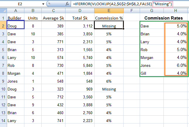
When we enter our formula in Excel, and apply it to the example we used for our VLOOKUP Exact Match example it would look like this:

=IFERROR(VLOOKUP(A2,$G$2:$H$8,2,FALSE),”Missing”)

You can see in the spreadsheet below that ‘Doug’ is no longer in our Commission Rates table and the IFERROR formula is telling Excel to put the word ‘Missing’ in the cell.

If we wanted Excel to put a number, say 0 in the cell instead of a word our formula would look like this.

=IFERROR(VLOOKUP(A2,$G$2:$H$8,2,FALSE),0)

You’ll notice the 0 doesn’t have inverted commas “ “ surrounding it like the text ‘Missing’ did.  The rule is if you want Excel to enter text you need to surround it in inverted commas, but for numbers you just enter them without the inverted commas.

To enter nothing, your formula would read:

=IFERROR(VLOOKUP(A2,$G$2:$H$8,2,FALSE),””)

To enter a dash – your formula would read:

=IFERROR(VLOOKUP(A2,$G$2:$H$8,2,FALSE),”-”)

Other uses for the IFERROR

As I mentioned above, the IFERROR can also hide #DIV/0!, #NAME?, #NULL!, #NUM!, #REF!, and #VALUE!

The other most common error is #DIV/0!  Let’s quickly look at how we’d hide this error by wrapping it in IFERROR.

Say we had a calculation that was =10/0 the result would be #DIV/0!.  To hide this we can wrap our formula in the IFERROR like this:

=IFERROR(10/0,”Error”) and instead of Excel displaying #DIV/0! it would display ‘Error’

Or if we wanted it to display 0 we’d enter the formula like this:

=IFERROR(10/0,0)

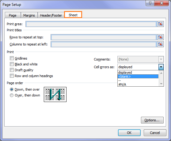
One last thing – Cell Error Print Options

What if you want to keep the errors in the spreadsheet and only hide them when printing?  Sometimes it’s useful to know where the errors are so you can correct any that are not expected, but if you regularly print reports you probably don’t want the errors displayed.

There’s a simple print setting that will allow you to define how errors are displayed when printing.  You can choose to either enter a — in the place of any errors, or leave the cell blank.

In the Page Setup on the Sheet tab choose how you want cell errors displayed from the drop down list.

Download the Excel workbook used in this example so you can copy and practice the IFERROR formula to make sure you really get it and can take advantage of its power.

Check out our other Excel Formulas Explained tutorials here, or for our Free Microsoft Office Online Training video tutorials click here to get over 10 hours of Excel, Word and Outlook training.

Tell us how you use IFERROR formulas in your work by entering a comment below.

Did you find this useful? Why not share the love and let your friends and colleagues know. Click the icons below for Twitter, facebook, Stumbleupon and many more.

Share This

Tweet

Please share this or leave a comment and I'll make sure you get a personal reply.

Tagged as: excel formulas, excel iferror formula